1. Title: Use of smith chart.
Aim:Use of Smith chart for transmission line pattern.
Objectives:
1) To Determine the Voltage reflection coefficient.
2) To Determine the VSWR.
3) To Determine the impedance Zx from load.
Introduction:
The Smith chart is one of the most useful graphical tools for high frequency circuit
applications. The chart provides a clever way to visualize complex functions.
The normalized impedance is represented on the Smith chart by using families of
curves that identify the normalized resistance r (real part) and the normalized reactance x
(imaginary part).
Zn = r + jx
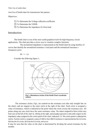
Consider the following figure 1,
The resistance circles, Fig1, are centred on the resistance axis (the only straight line on
the chart), and are tangent to the outer circle at the right of the chart. Each circle is assigned a
value of resistance, which is indicated at the point where the circle crosses the resistance axis. All
points along any one circle have the same resistance value. The values assigned to these circles vary
from zero at the left of the chart to infinity at the right, and actually represent a ratio with respect to the
impedance value assigned to the centre point of the chart, indicated 1.0. This centre point is called prime
centre. If prime centre is assigned a value of 100 Ω, then 200 Ω resistance is represented by the 2.0 circle,
50 Ω by the 0.5 circle, 20 Ω by the 0.2 circle, and so on.
It may be seen that the value on the chart is determined by dividing the actual resistance by the
number.

2. Suppose, we have an impedance consisting of 50 Ω resistance and 100 Ω inductive reactance
i.e. Zn = 50 + j 100.
If we have characteristicimpedance of 100 Ω to prime centre, we normalize
the above impedance by dividing each component of the impedance by 100. The normalized
impedance is then
( 50/100 )+ j (100/100) = 0.5 + j 1.0. This impedance is plotted on theSmith Chart at the
intersection of the 0.5 resistance circle andthe +1.0 reactance circle, as indicated in Fig 3.
Fig: 3

3. Example:
A lossless 100 Ω transmission line is terminated in a load impedance ZL= 50 + j75 Ω
Calculate;
a) Voltage reflection coefficient.
b) VSWR.
c) Impedance Zx from load at distance 0.35ƛ.
Find using formulae and MATLAB program
Soln
:
We have, Characteristics impedance Z0= 100+j0Ω
= 100 Ω
Load impedance ZL= 50+j75 Ω.
a) Voltage reflection coefficient is given by,
= = v
∴ v=
( ) ( )
( ) ( )
=
, Z1= √ + = √−50 + 75
∴Z1 = 90.138 Ω
1 = tan / = tan ∴ 1= < -56.30
and , Z2= √ + = √150 + 75
∴ Z2 = 167.70 Ω
2 = tan / = tan ∴ 2= < 26.56
Now, v=
˂ 1
˂ 2
=
. ˂ .
. ˂ .
∴ v = 0.537< - 83
Now A = a cos and B = a sin . We have a = 0.537 and = - 83.
∴ A = 0.537cos− 83= 0.06544 and B = 0.537 sin − 83 = - 0.5329
∴ C = A + Bj = 0.06544 - j 0.5329 Ω
v = √ + = (0.06544) + (−0.5329)
∴ v = 0.5369.
To calculate using smith chart, first normalize the impedance ZL by dividing it with
Characteristics impedance Z0. Therefore, Zn =
75
= 0.5 + j 0.75 Ω . Now locate this
point on smith chart . Take the distance from this point to the prime centre of smith chart

4. in compass, and measure the reading on reflection coefficient scale from centre to towards
generator.
b) VSWR: It is given by , VSWR =
| v|
| v|
=
|0.5369|
|0.5369|
∴ VSWR = 3.32
To calculate using smith chart, the distance from this point to the prime centre of smith chart
in compass, and draw a circle (called VSWR circle) with respect to prime centre on smith
chart. At the intersection of the VSWR circle and the resistance axis, from centre to right
hand side on resistance axis, this point gives value of VSWR. Or we can simply calculate it
on VSWR scale give below of smith chart.
c) Impedance Zx from load at distance 0.35λ :
We have, Zx = Z0
+ 0tan
0 + tan
Where,β = 2π and π =180° , x = distance from load.
∴ Zx = 100×
( ) ( )
( ) ( )
= 100×
( ) ( )
( ) ( )
= 100 ×
(50 + 75)− 137.64
(100+ 0)− (68.82+103.23 )
= 100 ×
50−62.64
203.23−68.82
∴ Zx = 31.0 – 19.0 j Ω
To find Zx from load, read the value of wavelength on the wavelength towards generator scale for
normalise impedance and draw straight line form centre through Zn. Add the given value of
wavelength in this value. Find the resultant value on the scale and joint the point of this line with
VSWR circle, this gives the value of Zx from load.
Observation table:
Obs
no.
Value of
Parameter
Using
MATLAB
Using
Smith chart
1. v 0.066667-0.53333j 0.06544 - 0.5329 j
2. VSWR 3.3242 3.32
3. Zx 31.4352 - 20.1767 j 31.0 - 19.0 j
Result: Studied, smith chart using MATLAB.

5. Program:
% programme for transmission line parameter using smith chart
clc;
clear;
close all;
a= input('Enter the real value of load Impedance ZL, a= ');
b=input('Enter the Immaginary value of load impedance ZL, b= ');
ZL= a+1i*b;
disp(['ZL= ',num2str(ZL),'ohm']);
a1= input('Enter the real value of characteristic Impedance Z0, a1= ');
b1=input('Enter the Immaginary value of characteristic impedance Z0, b1= ');
Z0= a1+1i*b1;
disp(['Z0= ',num2str(Z0),'ohm']);
disp('Enter the R- To Determine the Voltage reflection coefficient');
disp('Enter the V- To Determine the VSWR');
disp('Enter the Z- To Determine the impedance Zx from load');
c = input('Enter your choice','s');
switch c
case 'R'
rc=(ZL-Z0)/(ZL+Z0);
disp(['The Voltage reflection coefficient is' ,num2str(rc)]);
case 'V'
rc=(ZL-Z0)/(ZL+Z0);
x=real(rc);
y=imag(rc);
q=sqrt(x^2+y^2);
VSWR=(1+q)/(1-q);
disp(['The VSWR is' ,num2str(VSWR)]);
case 'Z'
zx= Z0*((ZL+1i*Z0*tan((2*pi)*0.35))/(Z0+1i*ZL*tan((2*pi)*0.35)));
disp(['The Zx from load ZL is ' ,num2str(zx),'ohm']);
otherwise
error('invalid choice');
end