Downloaded 361 times
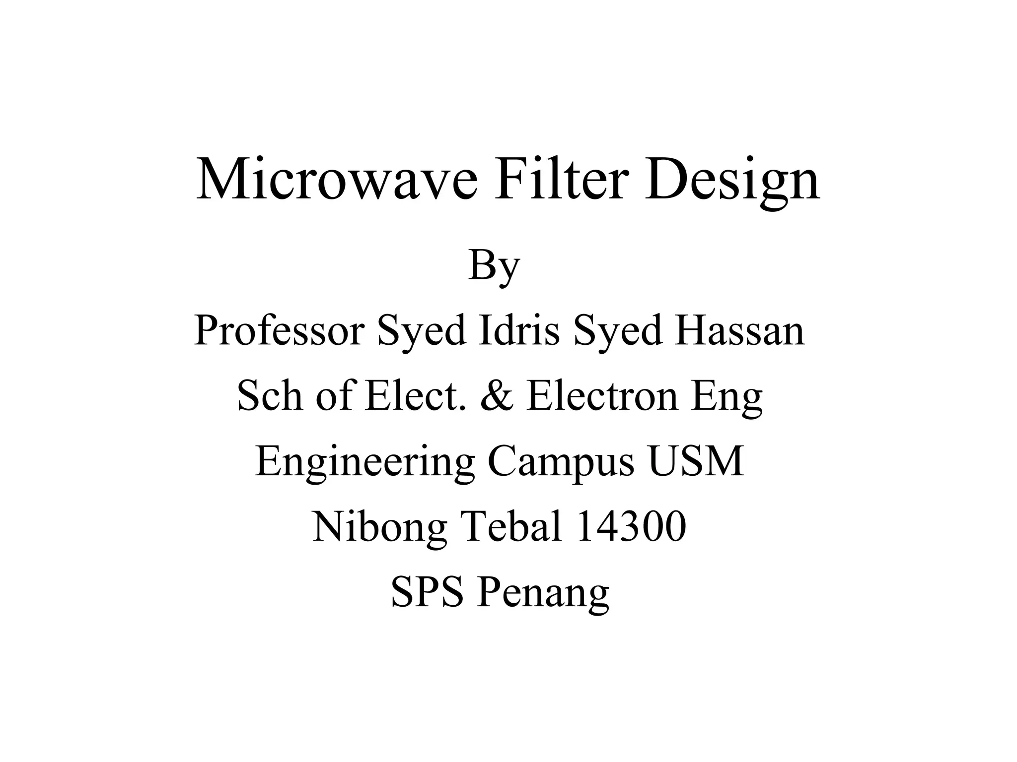
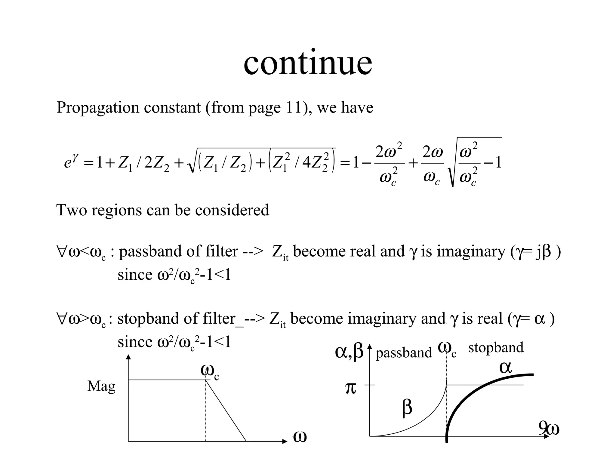
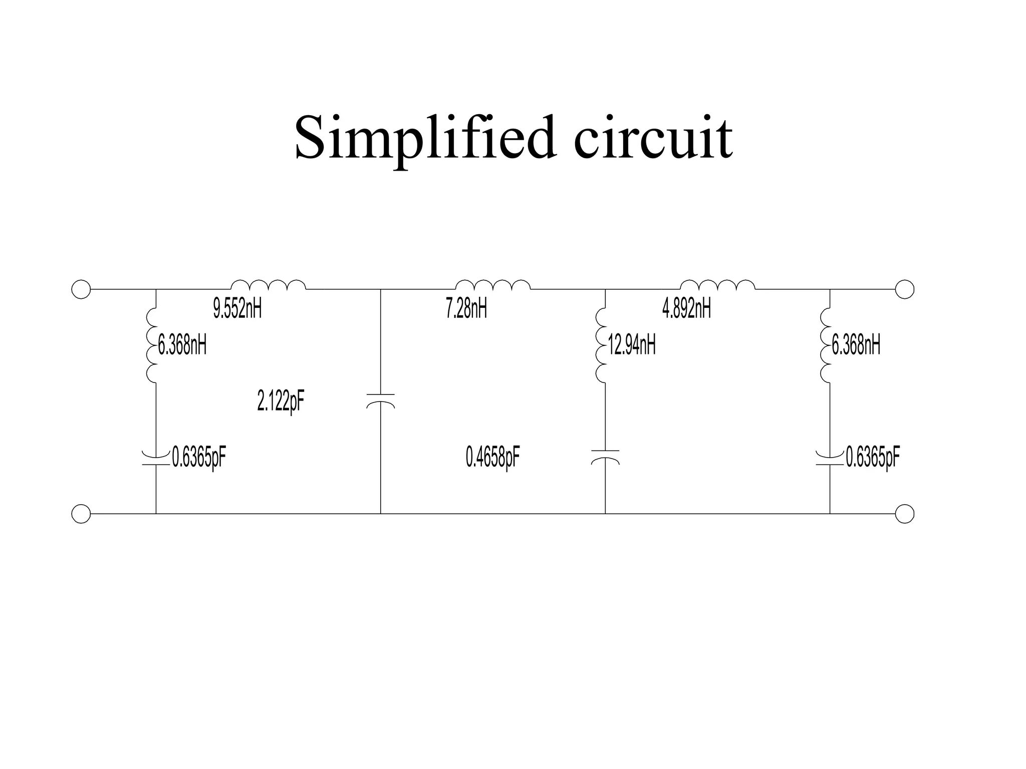

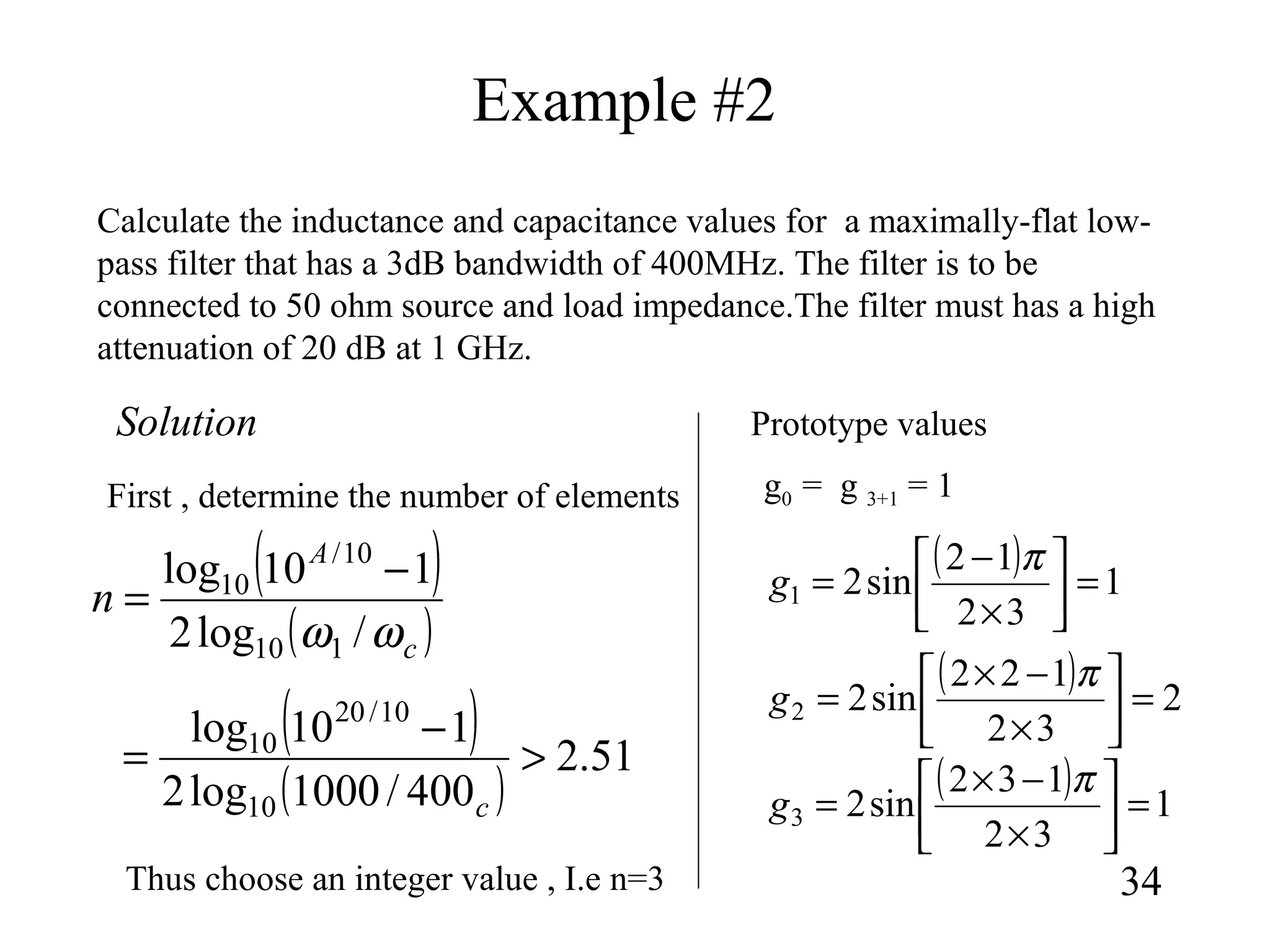

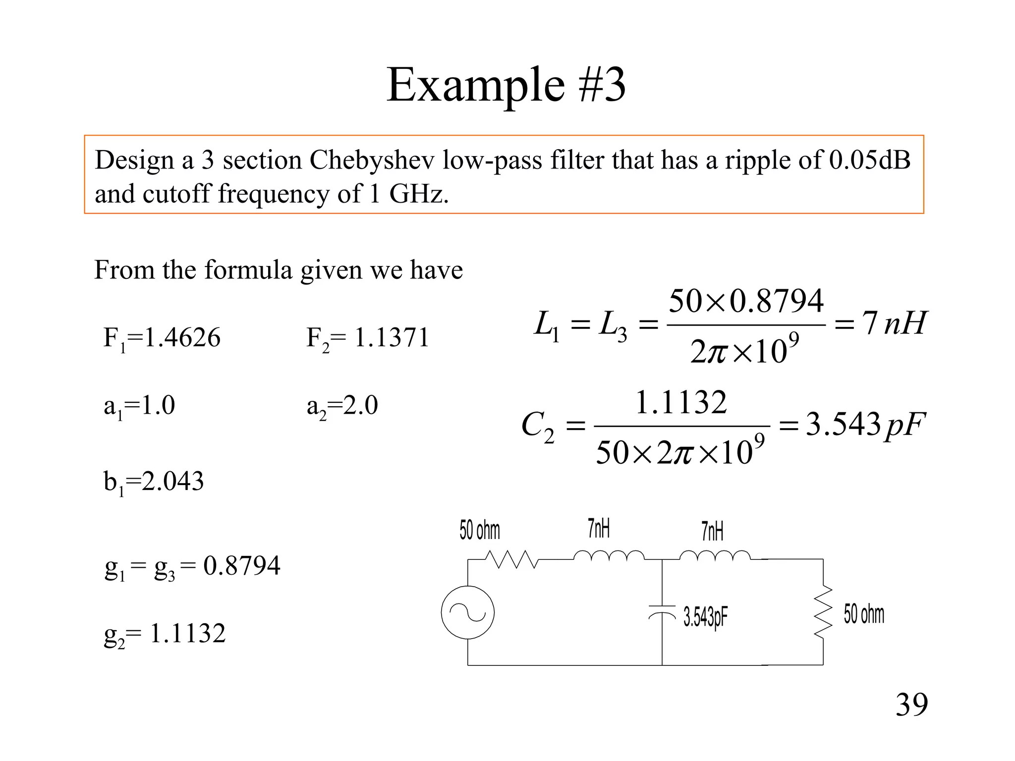
![Required admittance inverter parameters
58
2
1
10
01
2
'
Ω
=
gg
J
π
1,...2,1
1
2
'
1
1, −=×
Ω
=
+
+ nkfor
gg
J
kk
kk
π
tionsofnon
gg
J
nn
nn sec.
2
'
2
1
1
1, =
Ω
=
+
+
π
oω
ωω 12 −
=Ω
The normalized admittance inverter is given by
[ ]2
1,1,1, ''1, +++ ++= kkkkokkoe JJZZ
[ ]2
1,1,1,, ''1 +++ +−= kkkkokkoo JJZZ
okkkk ZJJ 1,1,' ++ =where
where A
B
C
D
E](https://image.slidesharecdn.com/filterdesign1-150319013708-conversion-gate01/75/Filter-design1-58-2048.jpg)
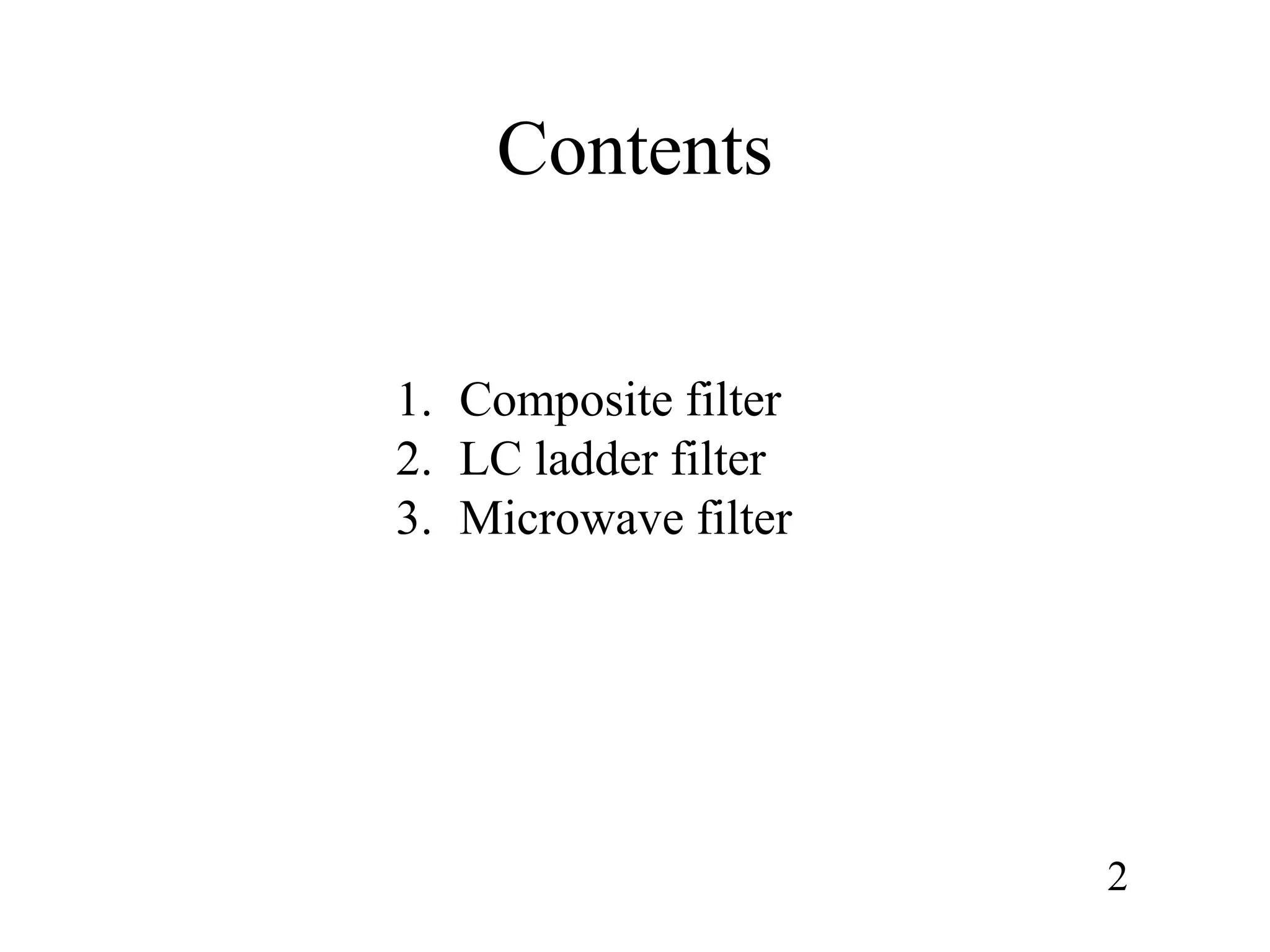
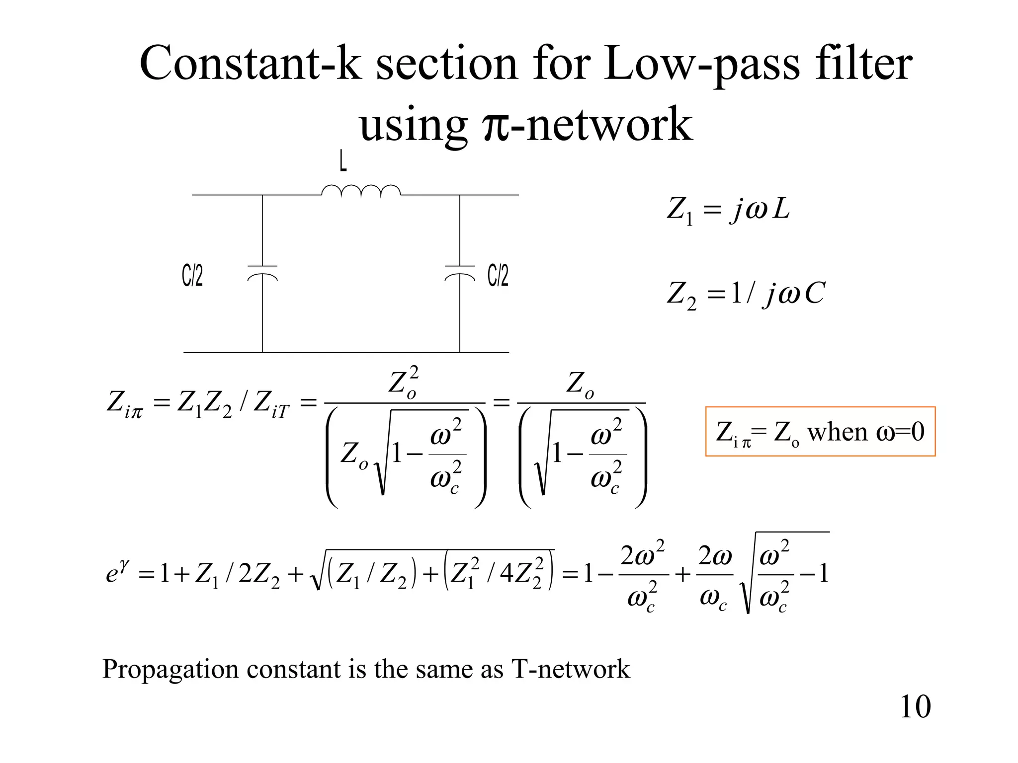
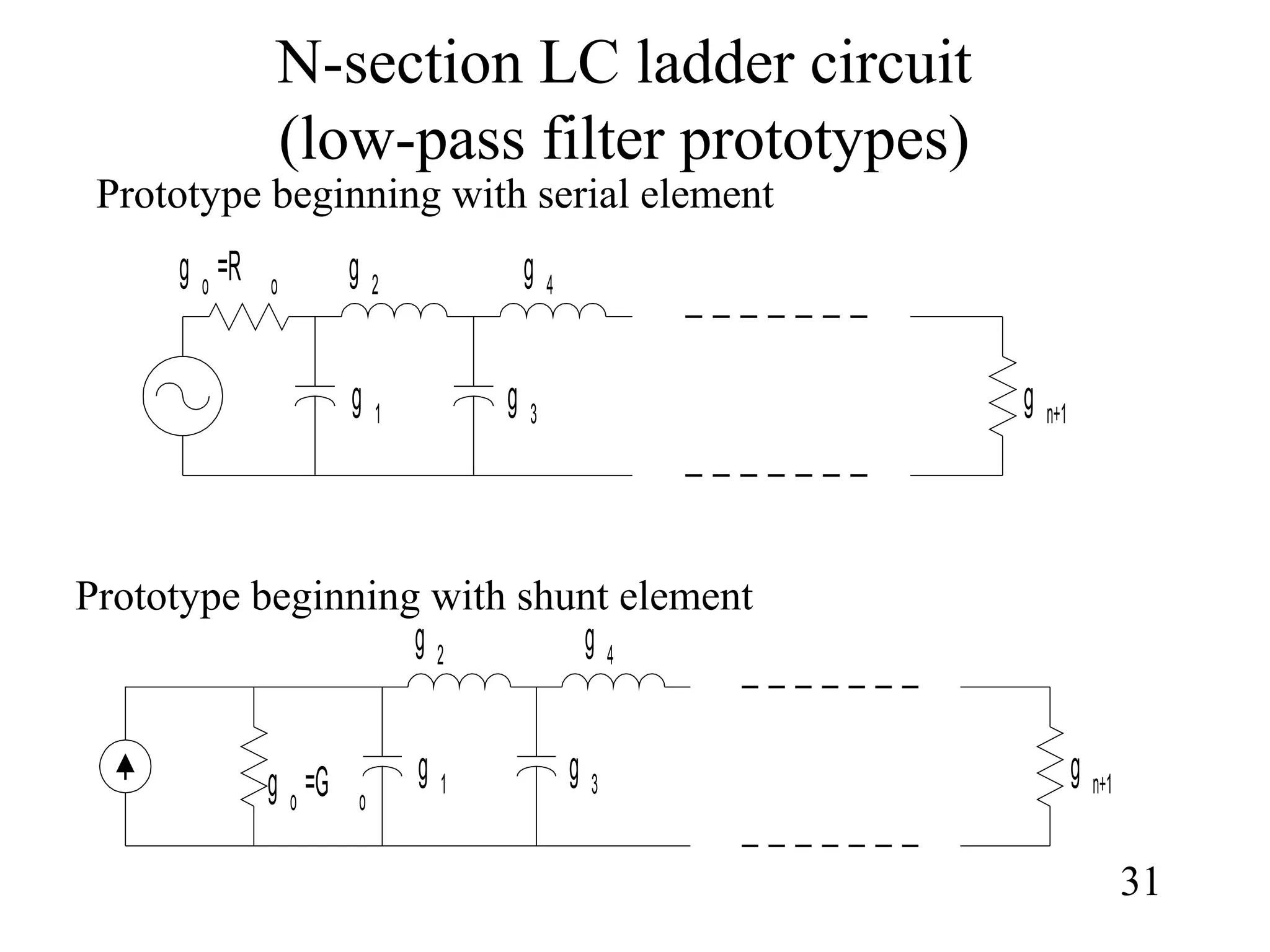
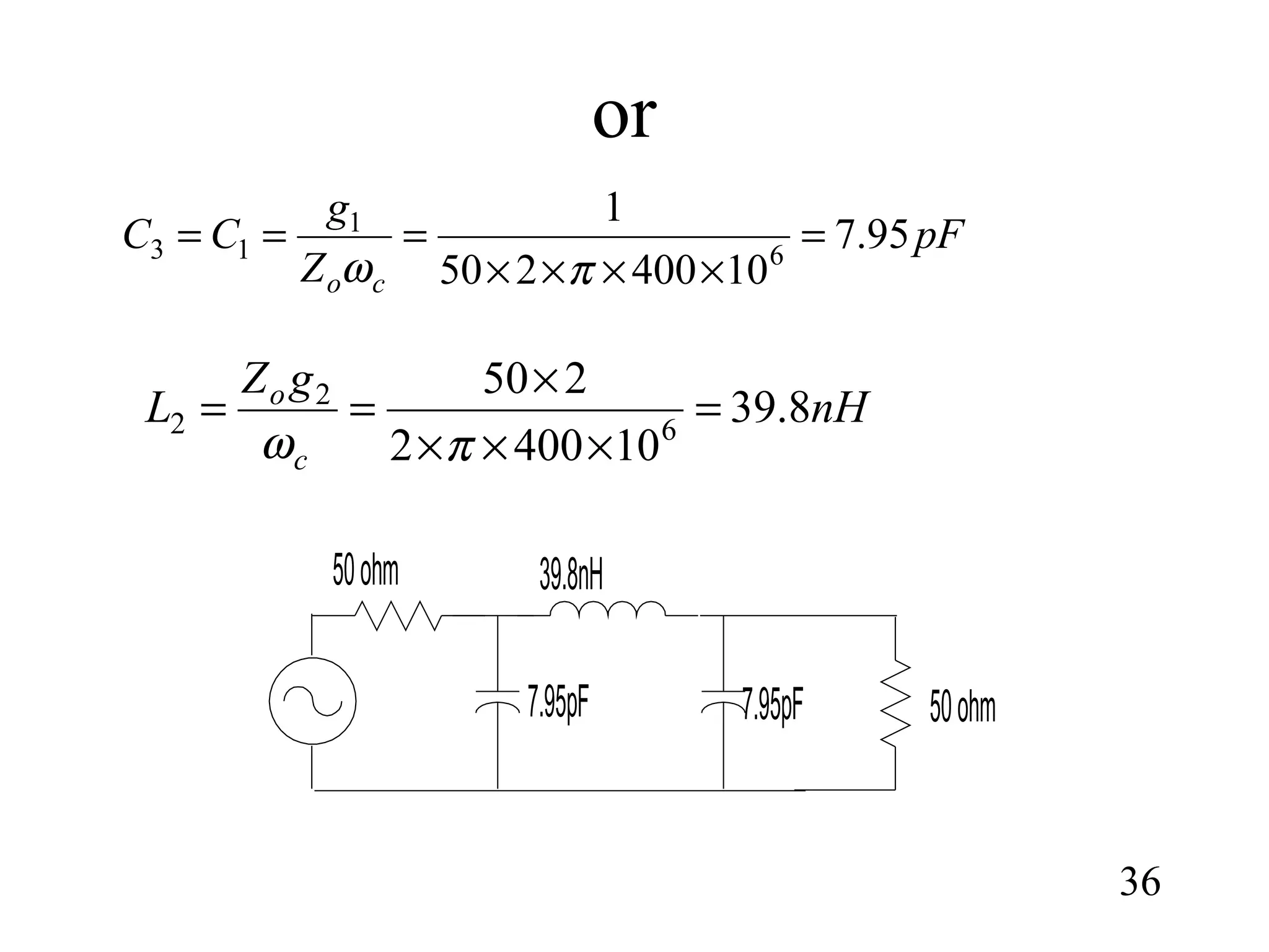
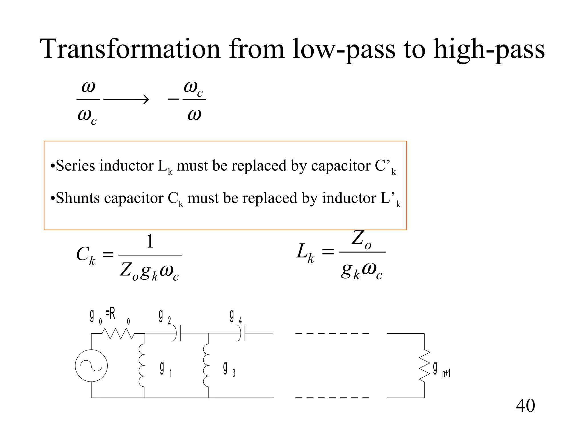
![Example #7
59
Design a coupled line bandpass filter with n=3 and a 0.5dB equi-ripple
response on substrate er=10 and h=1mm. The center frequency is 2 GHz, the
bandwidth is 10% and Zo=50Ω.
We have g0=1 , g1=1.5963, g2=1.0967, g3=1.5963, g4= 1 and Ω=0.1
3137.0
5963.112
1.0
2
'
2
1
2
1
10
01 =
××
×
=
Ω
=
ππ
gg
J
[ ] Ω=++== 61.703137.03137.0150,, 2
4,31,0 oeoe ZZ
[ ] Ω=+−== 24.393137.03137.0150 2
4,3,1,0, oooo ZZ
3137.0
15963.12
1.0
2
'
2
1
2
1
43
4,3 =
××
×
=
Ω
=
ππ
gg
J
A
C
D
E](https://image.slidesharecdn.com/filterdesign1-150319013708-conversion-gate01/75/Filter-design1-59-2048.jpg)
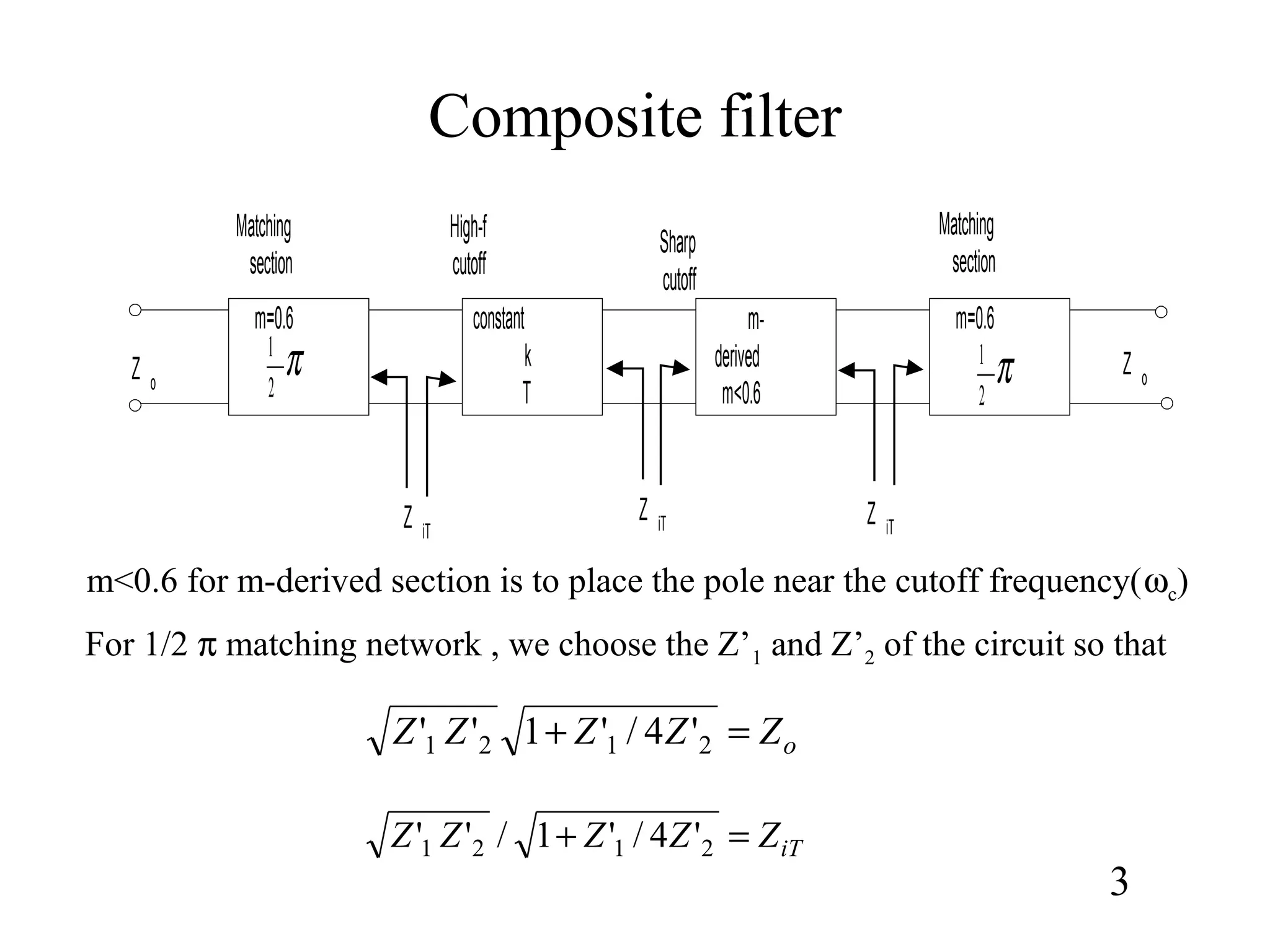
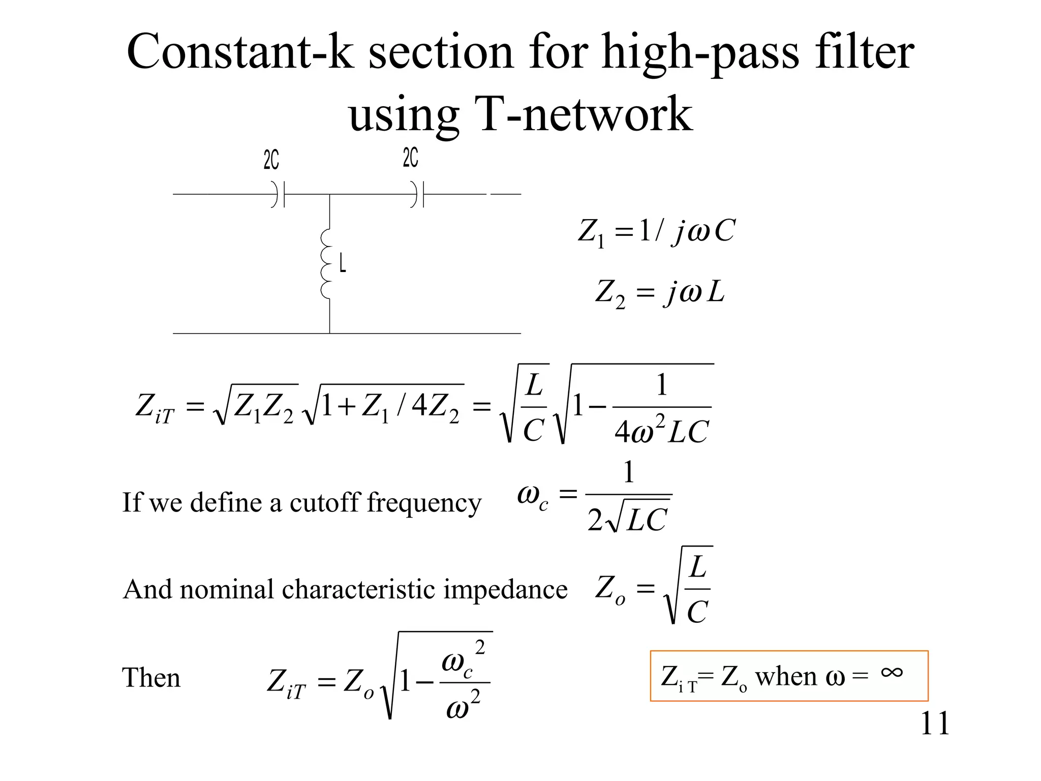
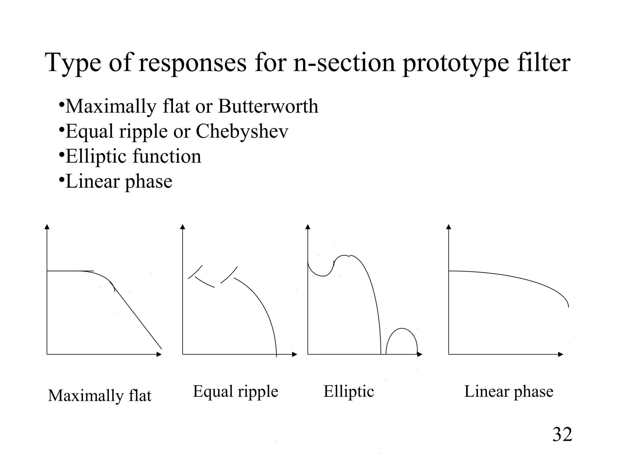
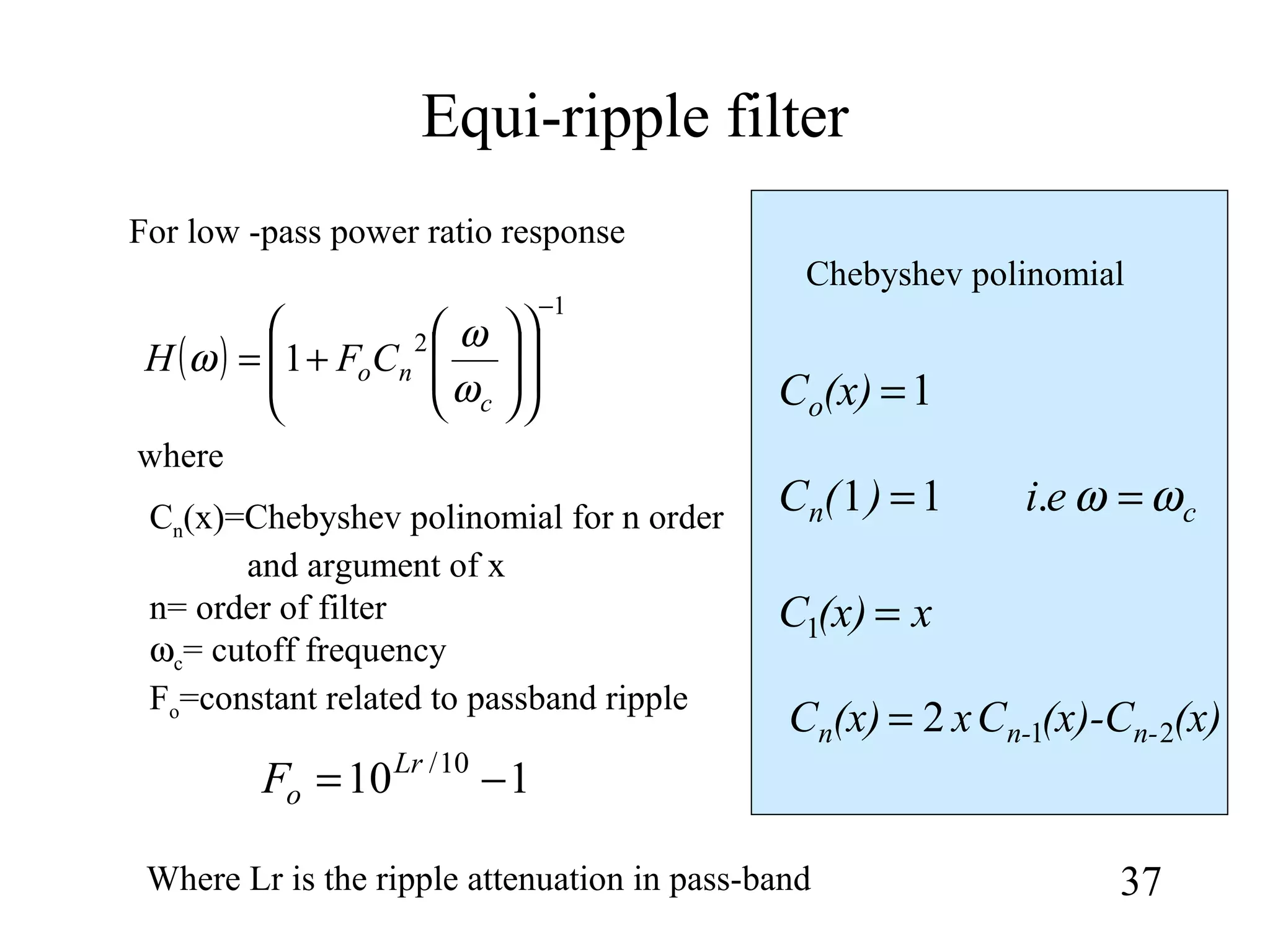
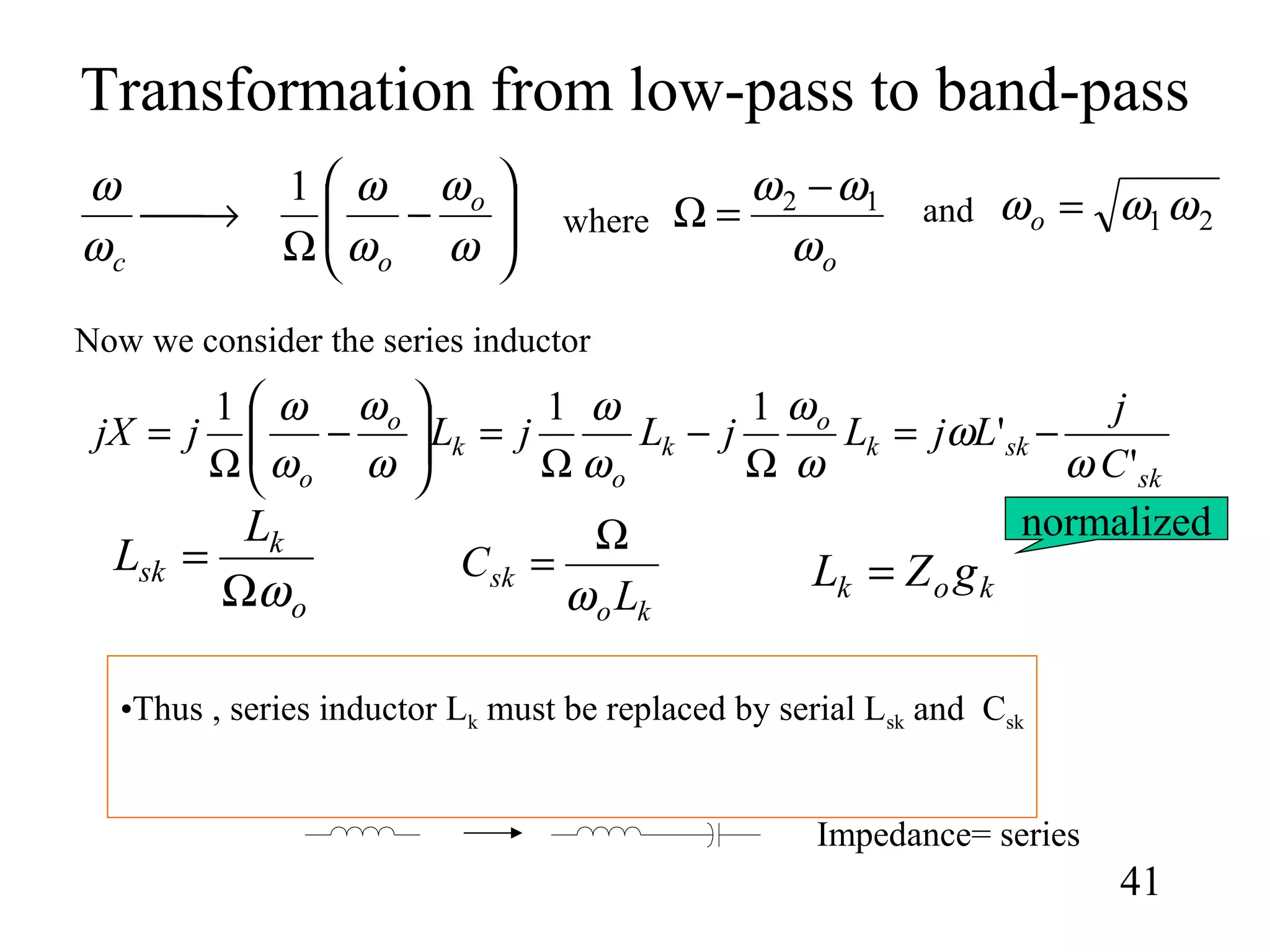
![60
1187.0
0967.15963.1
1
2
1.01
2
'
21
2,1 =
×
×
×
=×
Ω
=
ππ
gg
J
1187.0
5963.10967.1
1
2
1.01
2
'
32
3,2 =
×
×
×
=×
Ω
=
ππ
gg
JB
B
[ ] Ω=++== 64.561187.01187.0150,, 2
3,22,1 oeoe ZZ
[ ] Ω=+−== 77.441187.01187.0150 2
3,2,2,1, oooo ZZ
D
E
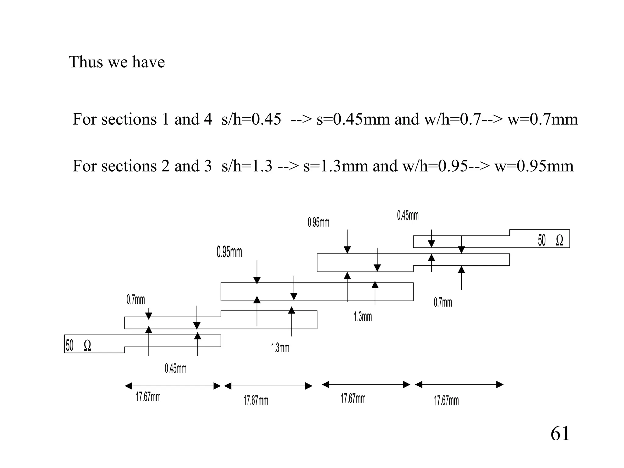
Using the graph Fig 7.30 in Pozar pg388 we would be able to determine the
required s/h and w/h of microstripline with εr=10. For others use other means.
m
f r
r 01767.0
101024
103
2
103
4/ 9
88
=
××
×
=
×
=
ε
λThe required resonator](https://image.slidesharecdn.com/filterdesign1-150319013708-conversion-gate01/75/Filter-design1-60-2048.jpg)


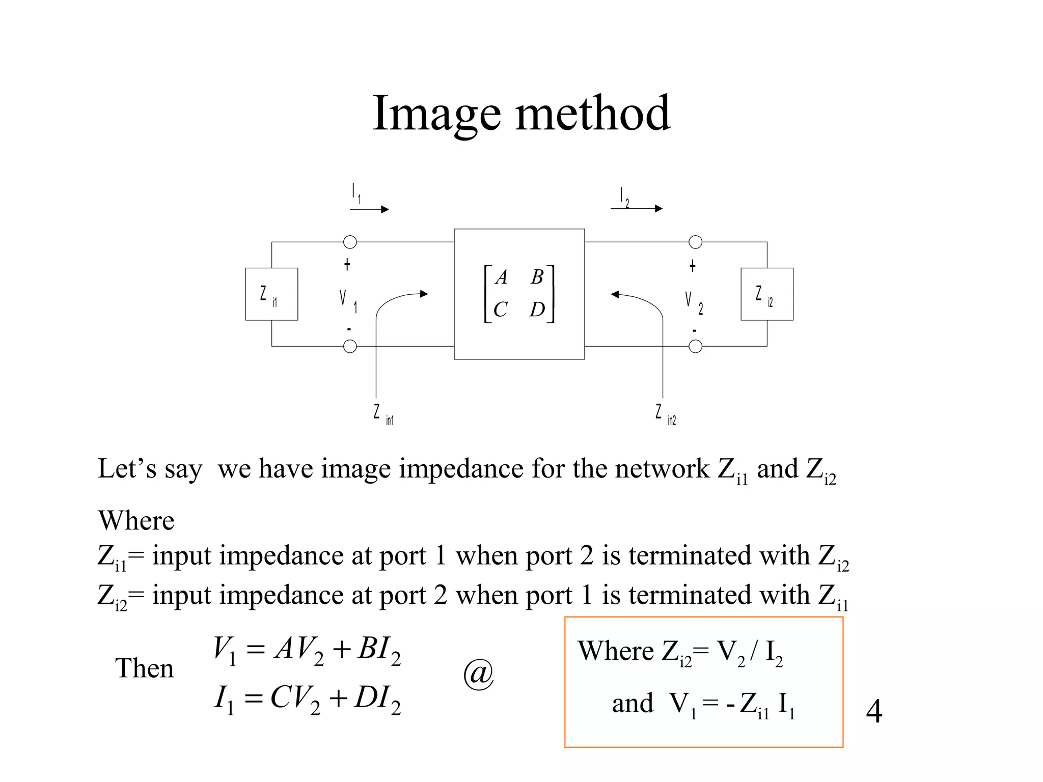
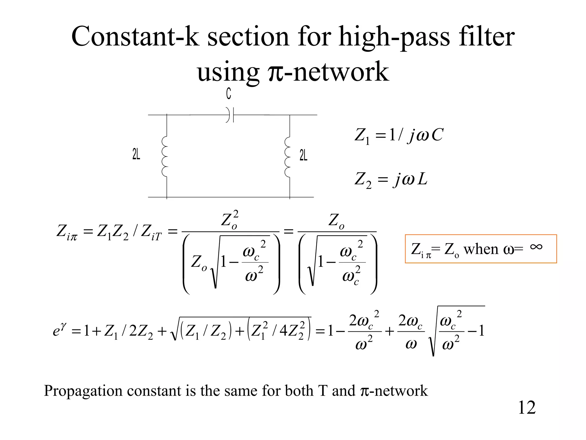
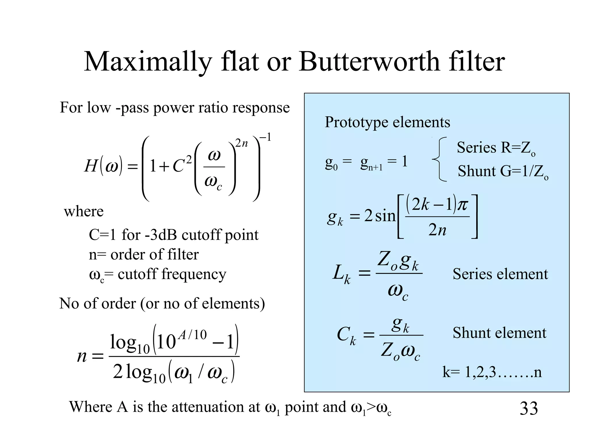
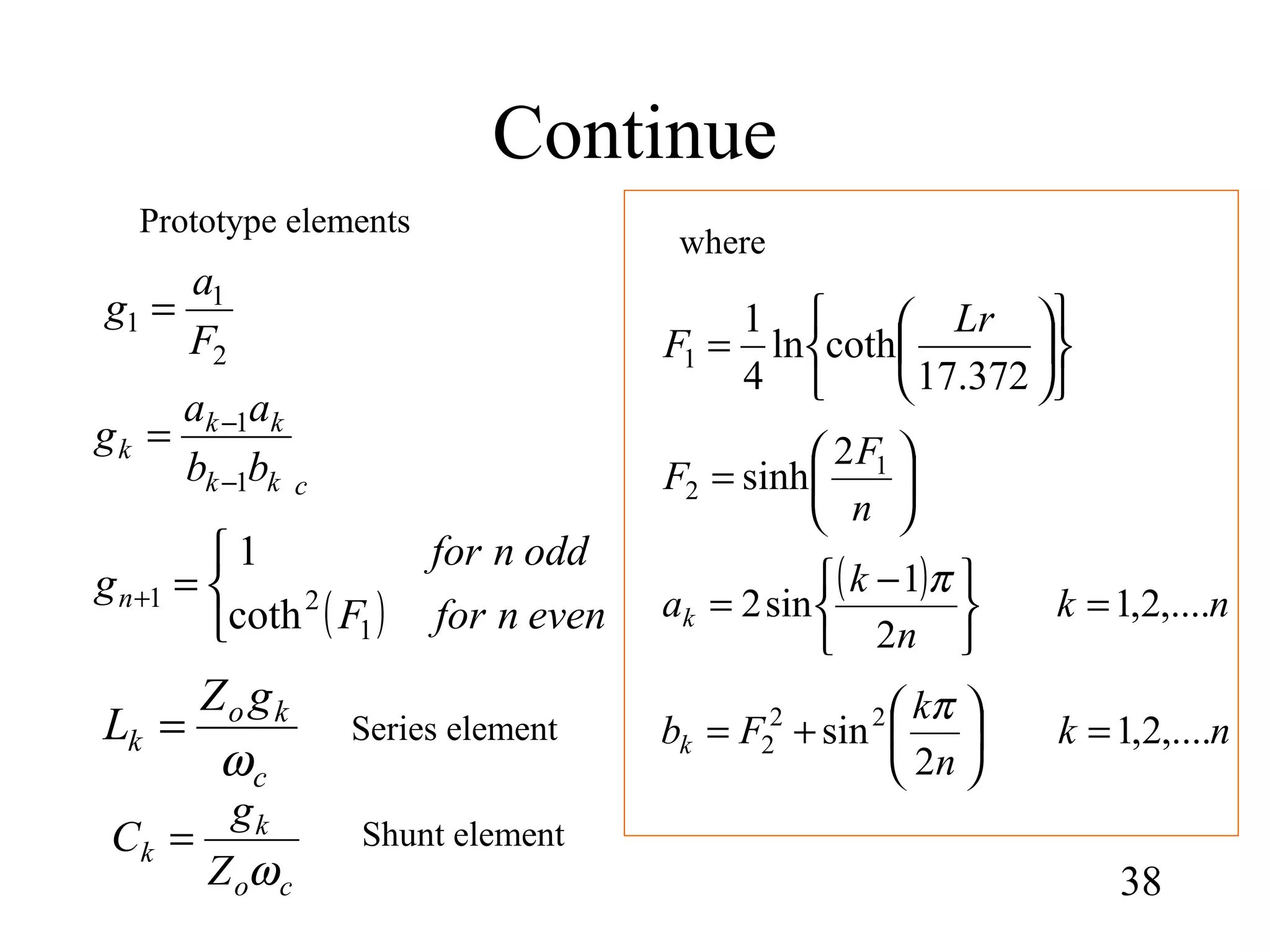
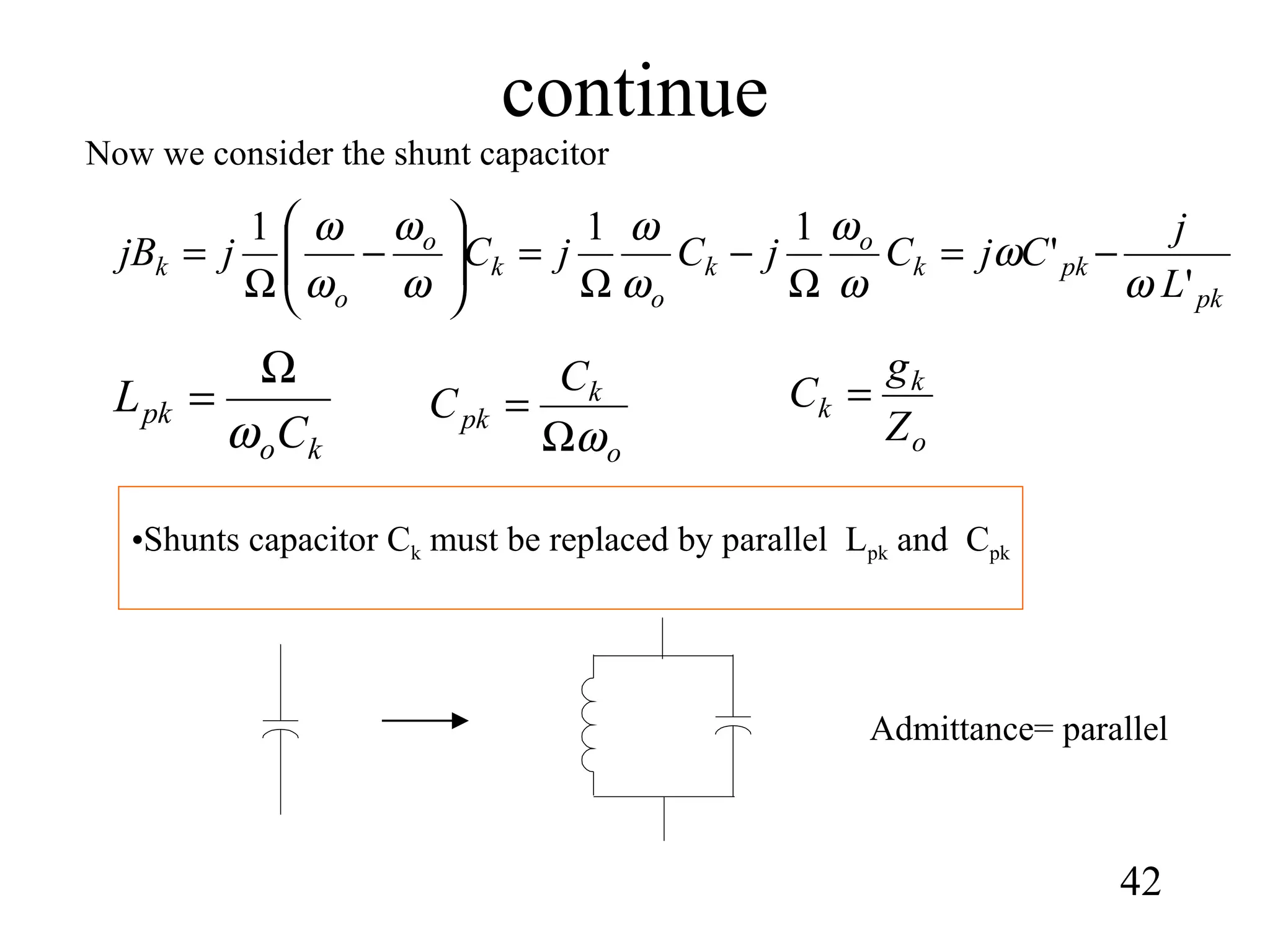
![Capacitive coupled resonator band-pass filter
64
Z o Z oZ oZ o
....
B 2B 1
θ 2θ 1
B n+1
Z o
θ n
2
1
10
01
2
'
Ω
=
gg
J
π
1,...2,1
1
2
'
1
1, −=×
Ω
=
+
+ nkfor
gg
J
kk
kk
π
tionsofnon
gg
J
nn
nn sec.
2
'
2
1
1
1, =
Ω
=
+
+
π
oω
ωω 12 −
=Ωwhere
( )2
1 io
i
i
JZ
J
B
−
=
( )[ ] ( )[ ]1
11
2tan
2
1
2tan
2
1
+
−−
++= ioioi BZBZπθ
i=1,2,3….n](https://image.slidesharecdn.com/filterdesign1-150319013708-conversion-gate01/75/Filter-design1-64-2048.jpg)
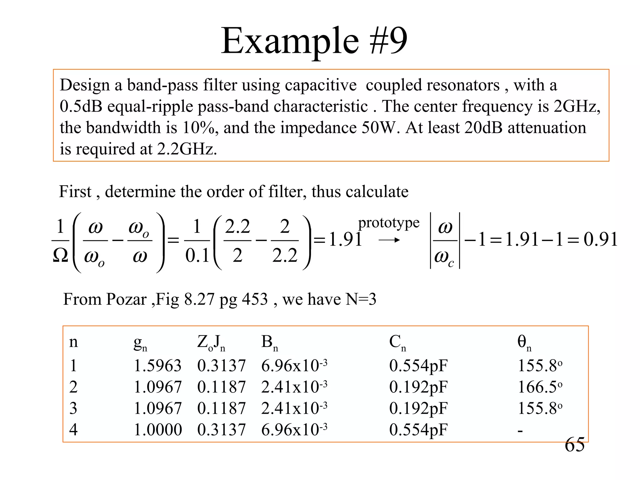

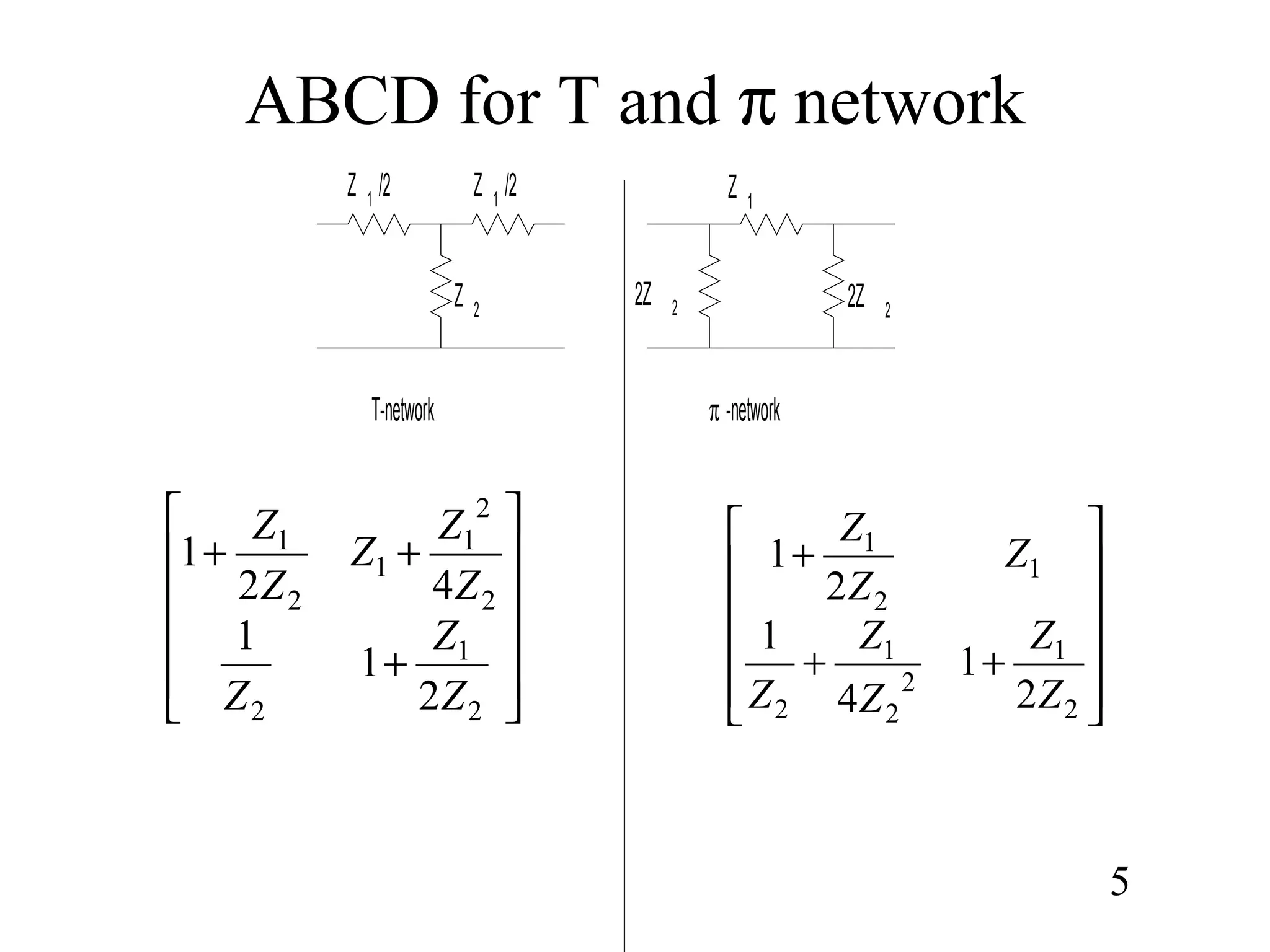
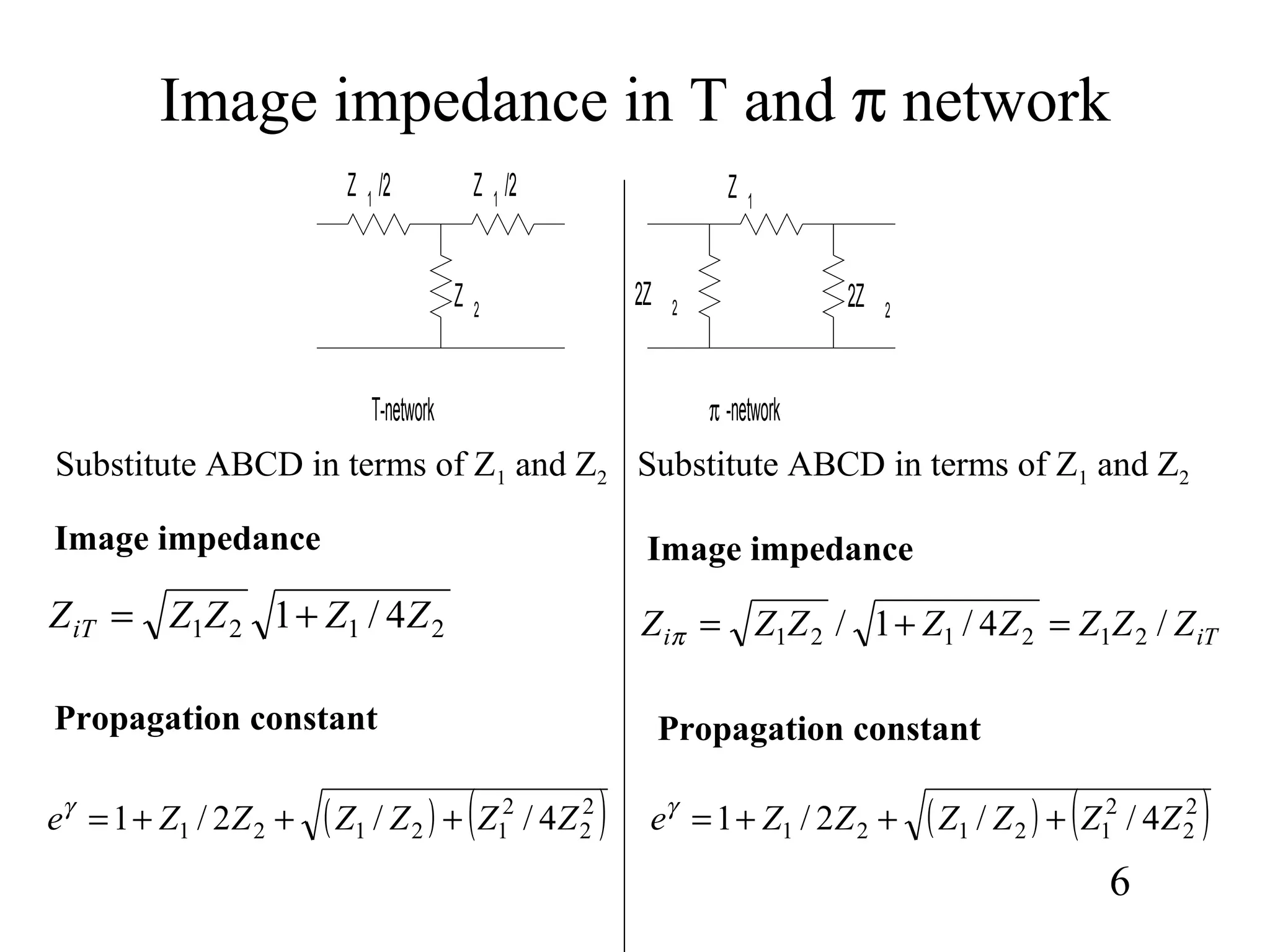
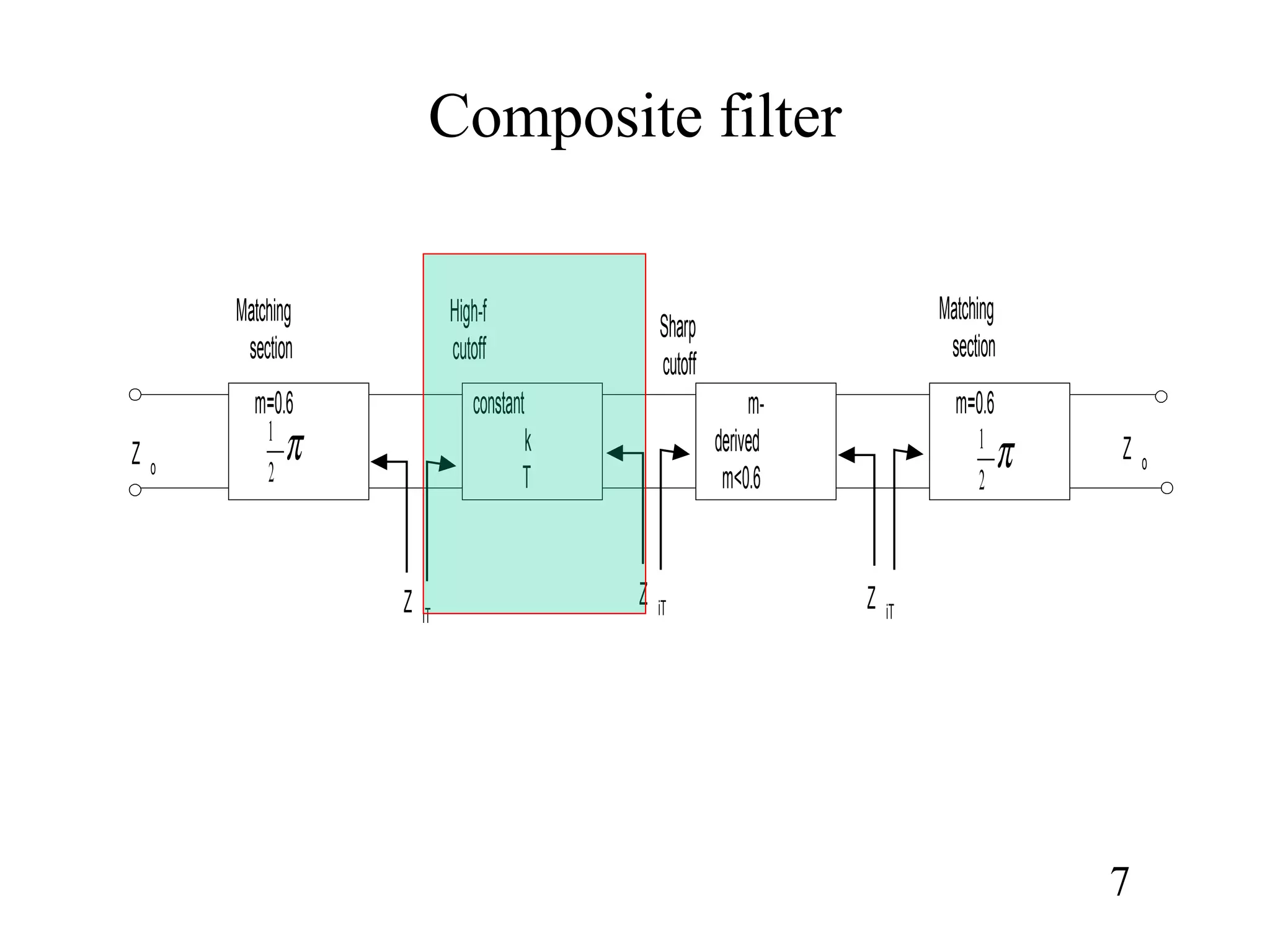
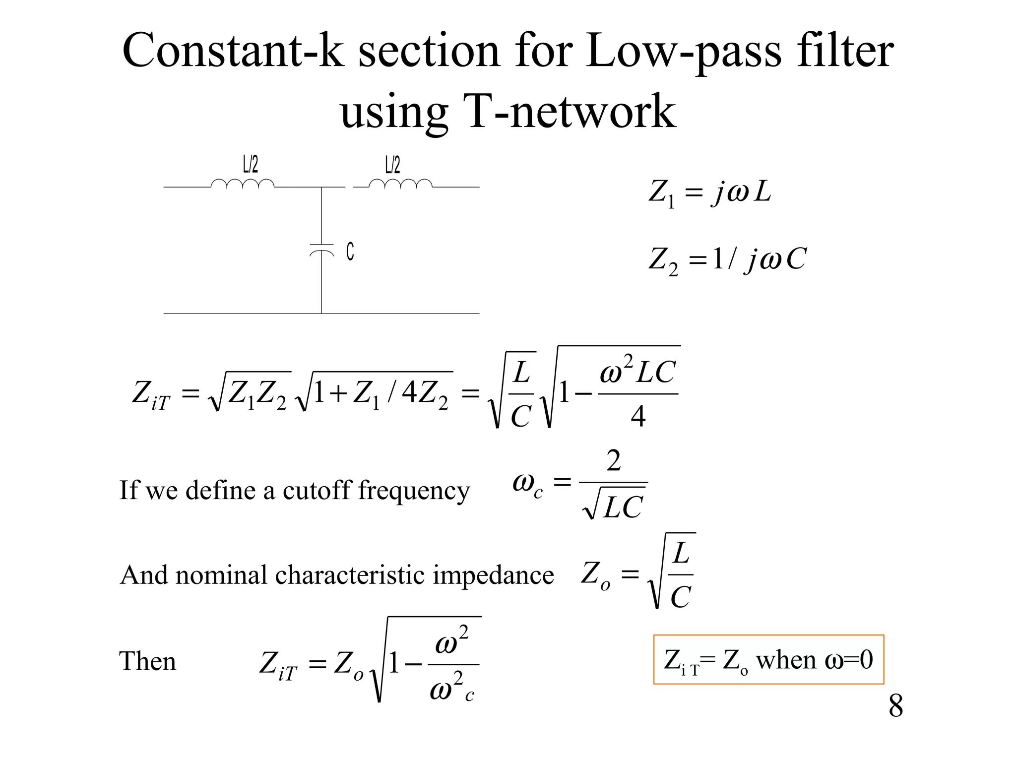
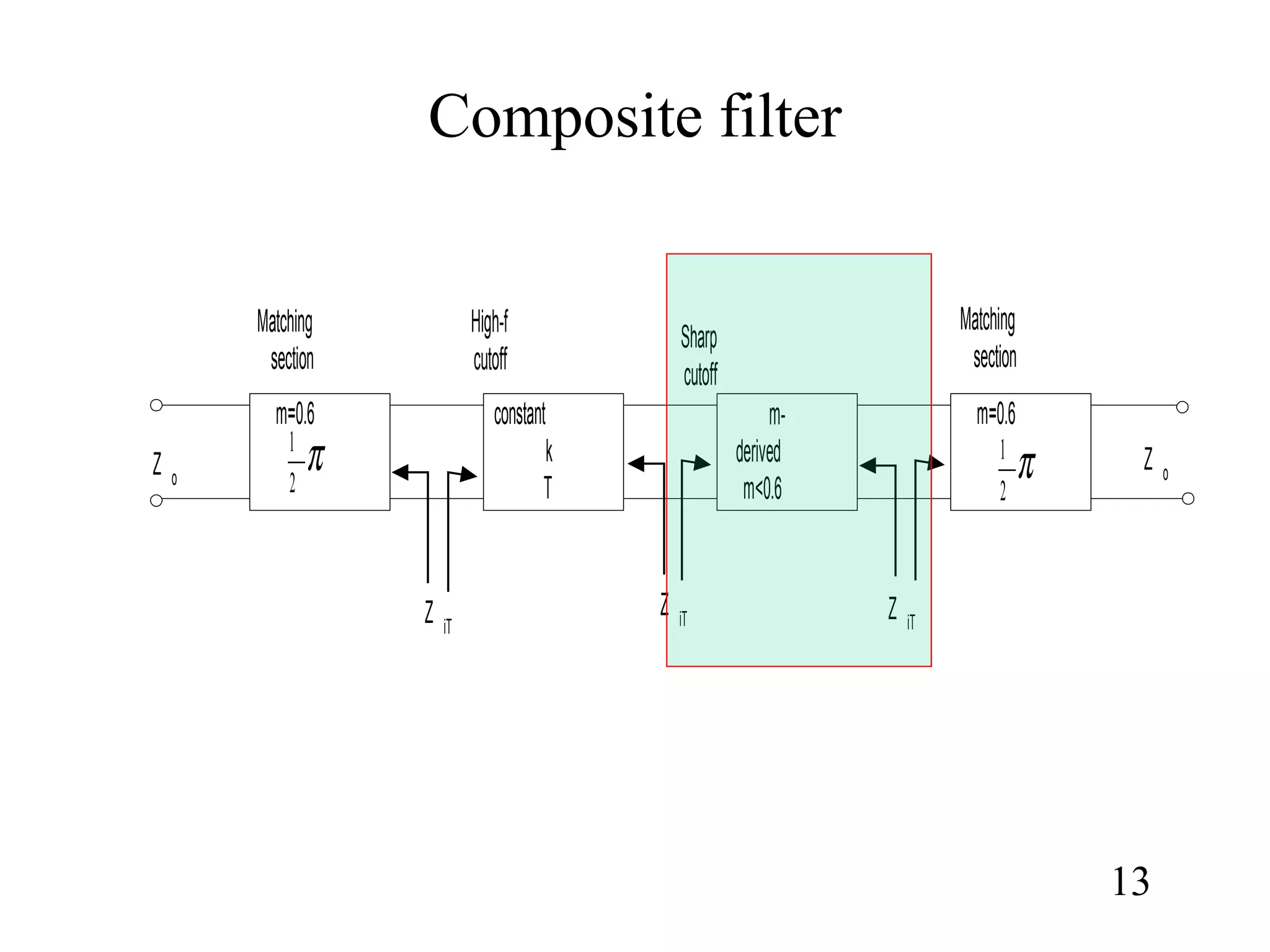
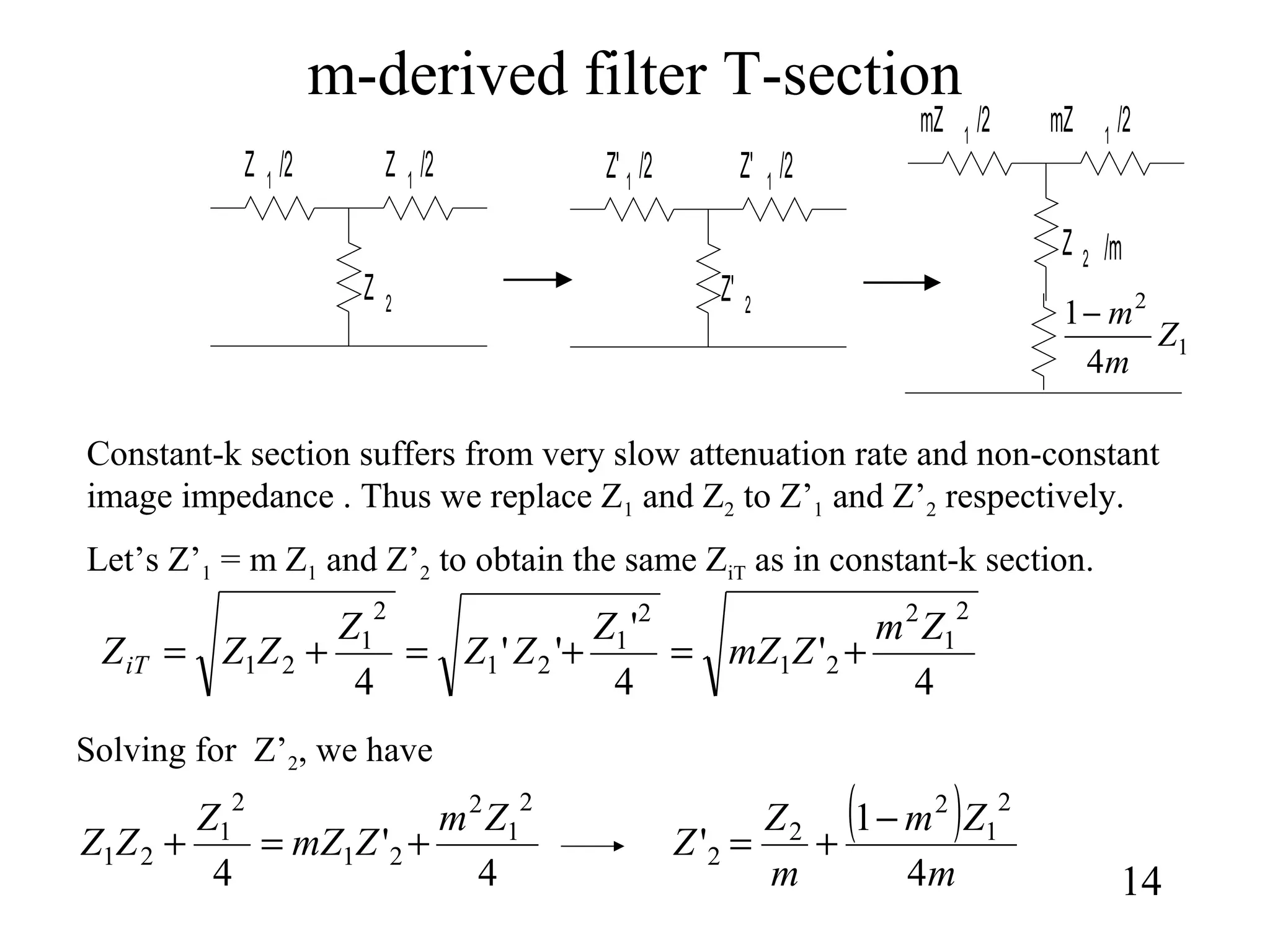
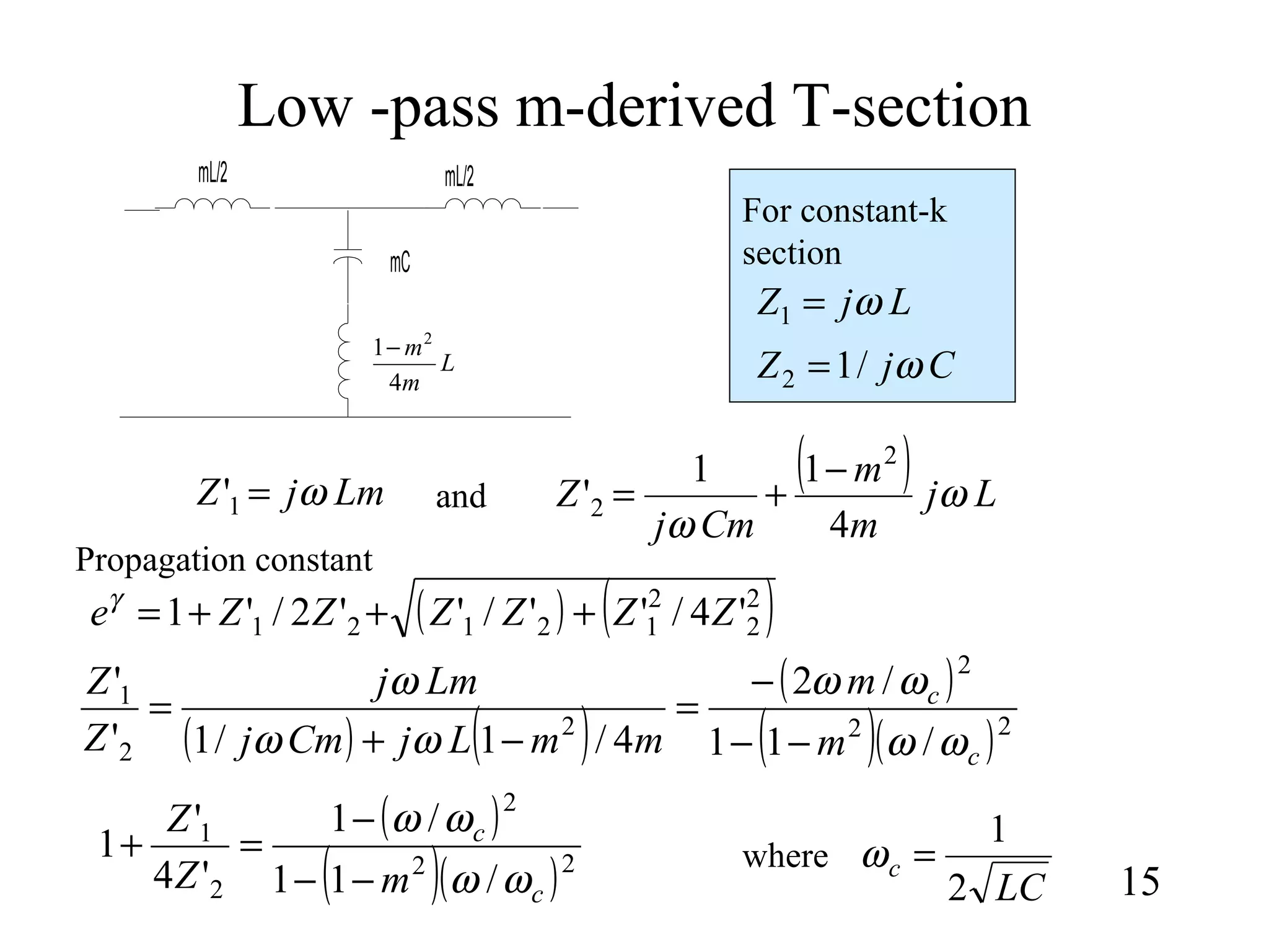
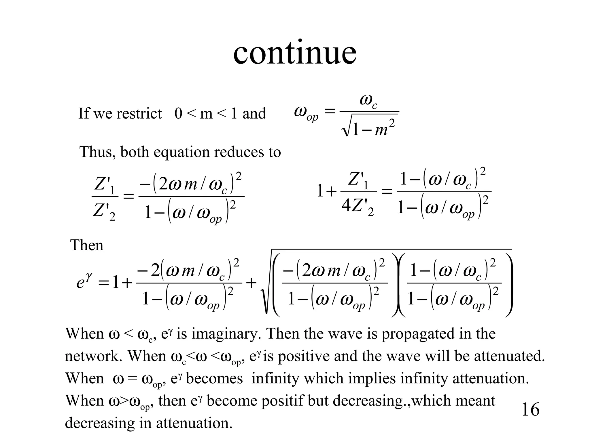
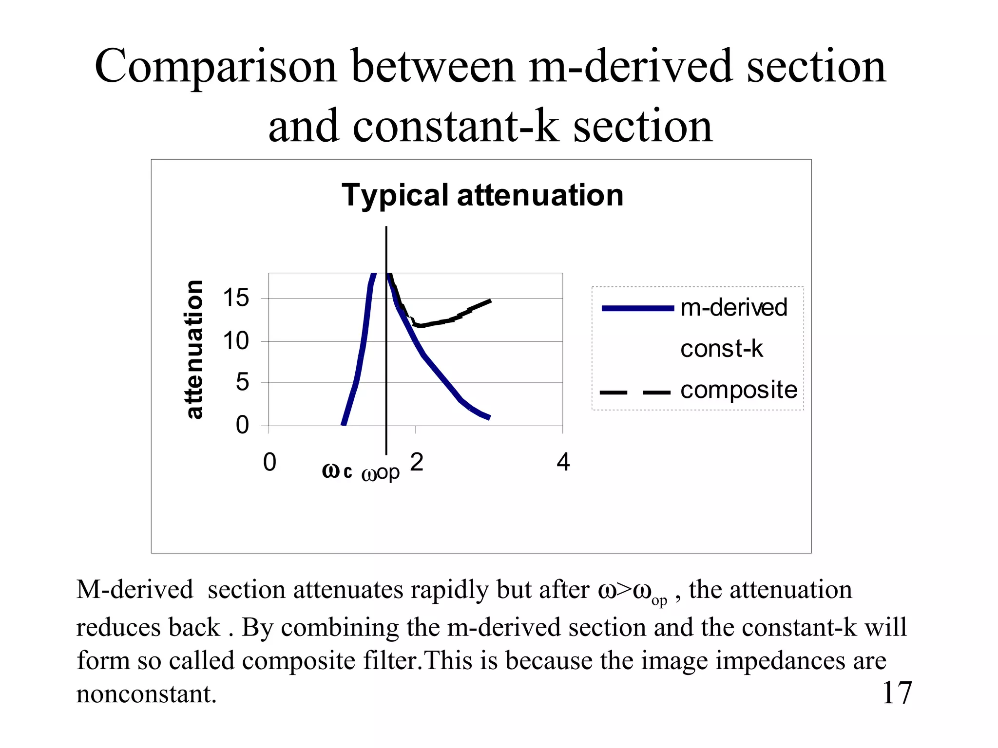
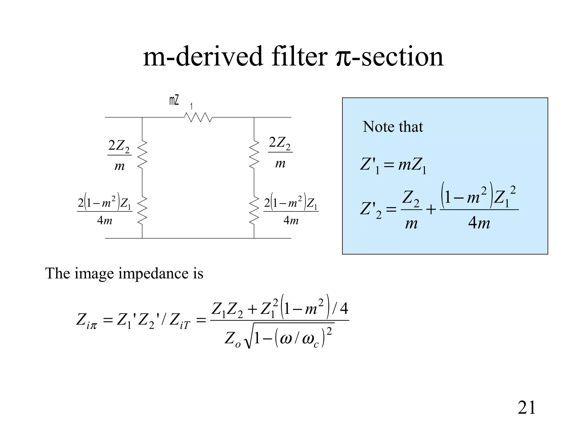
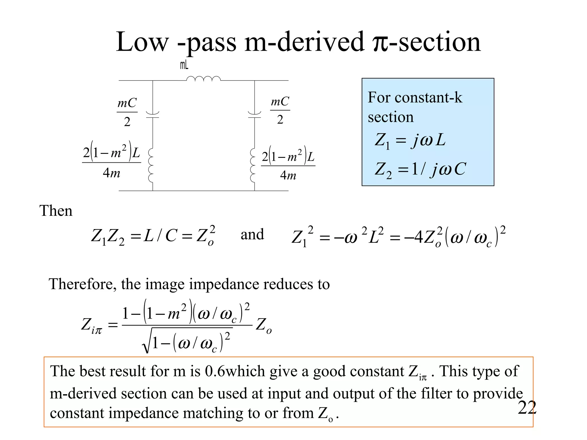
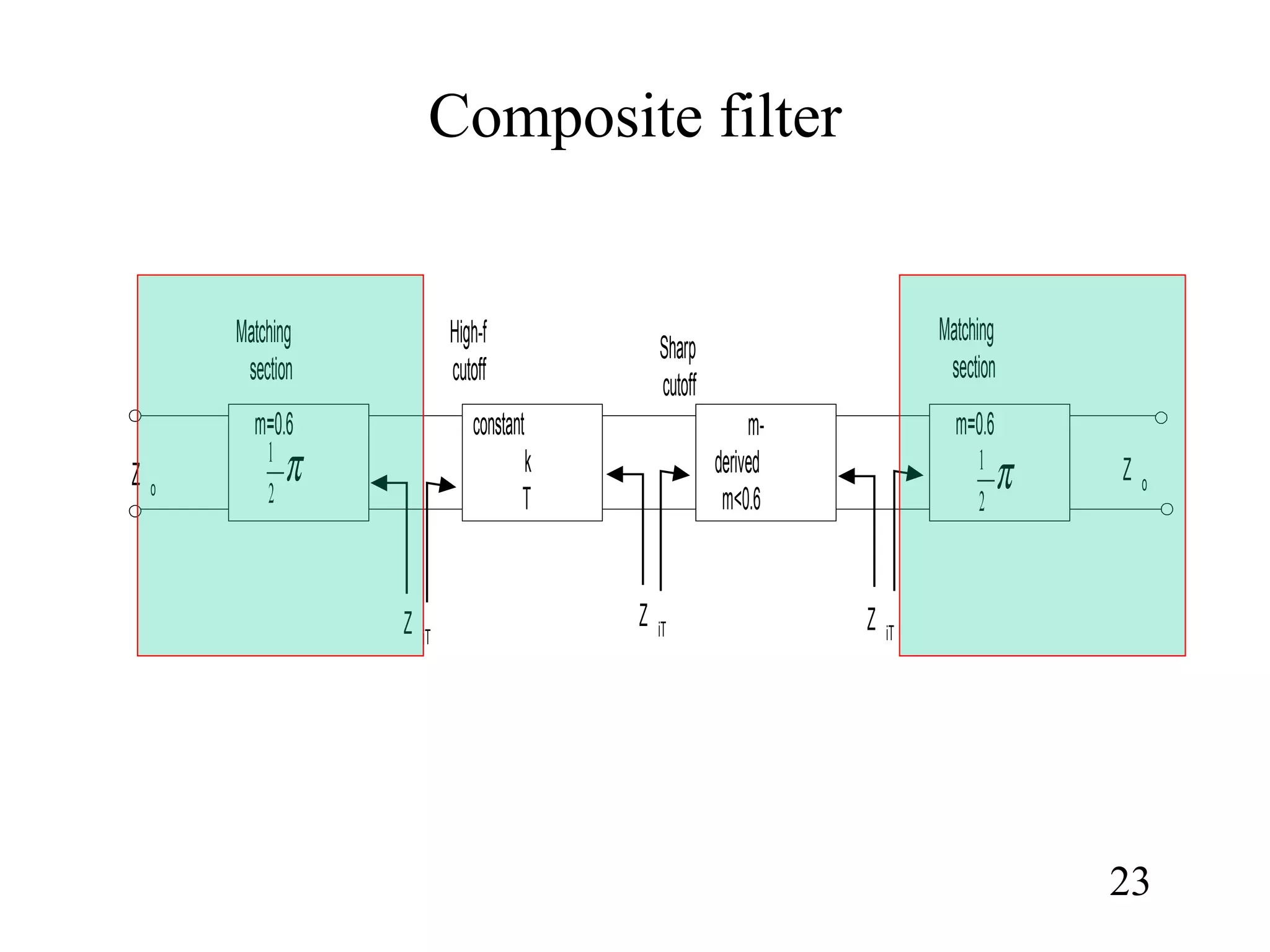
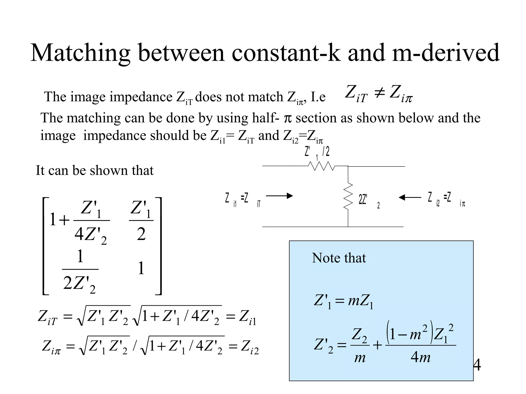
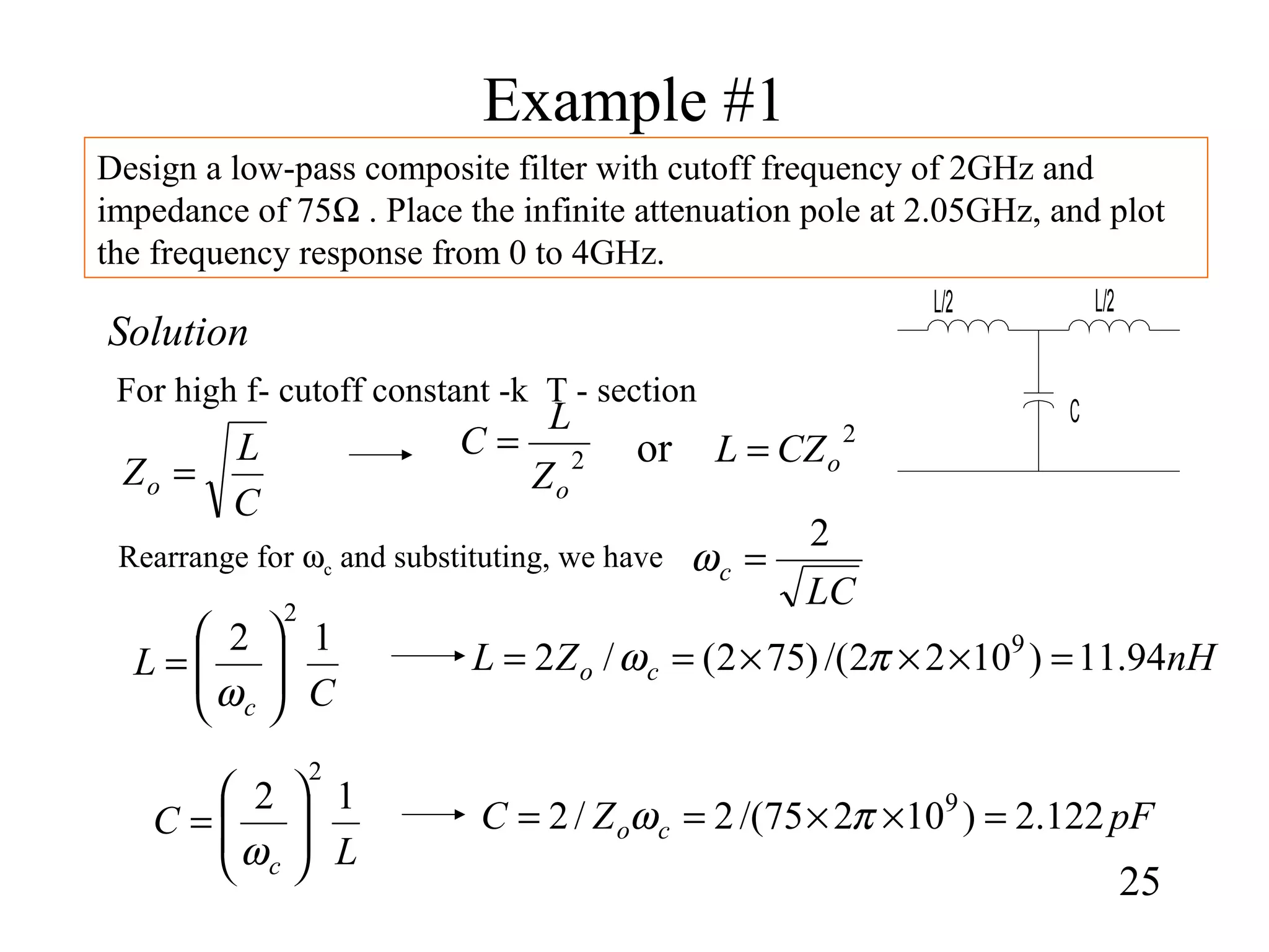
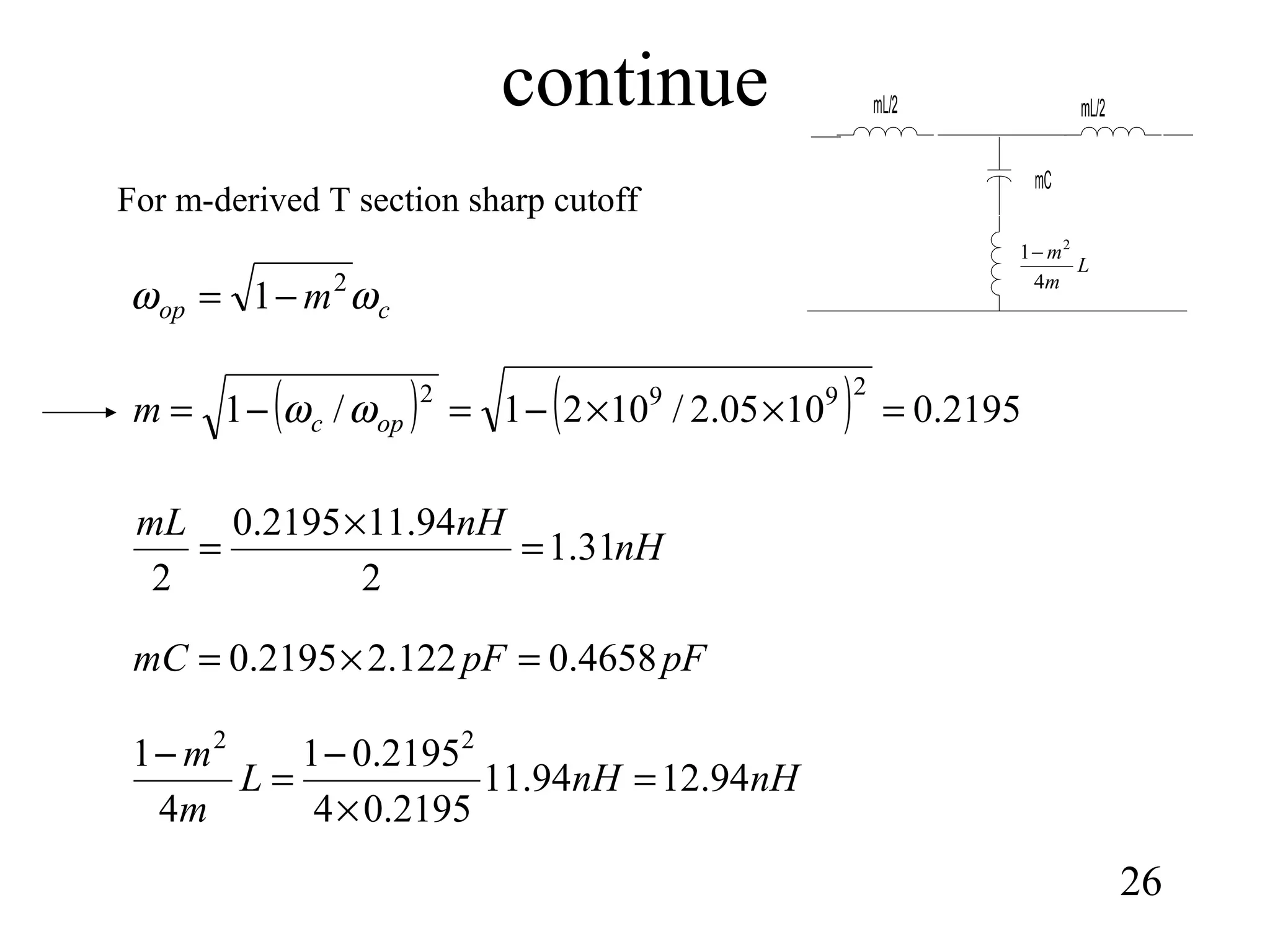
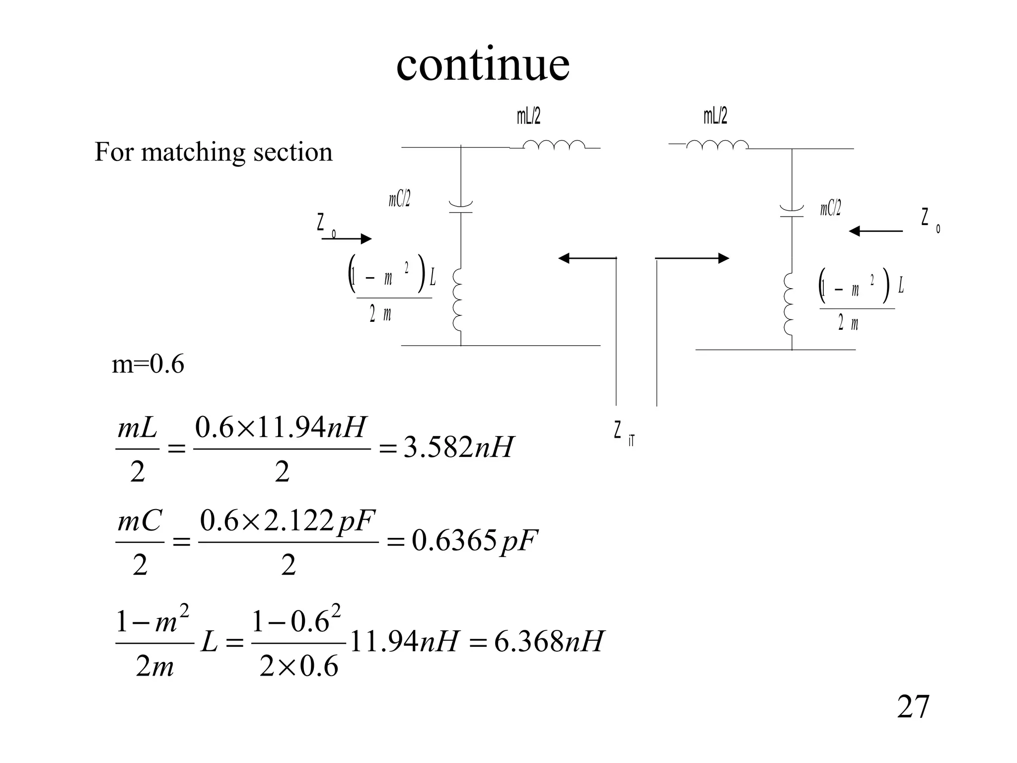
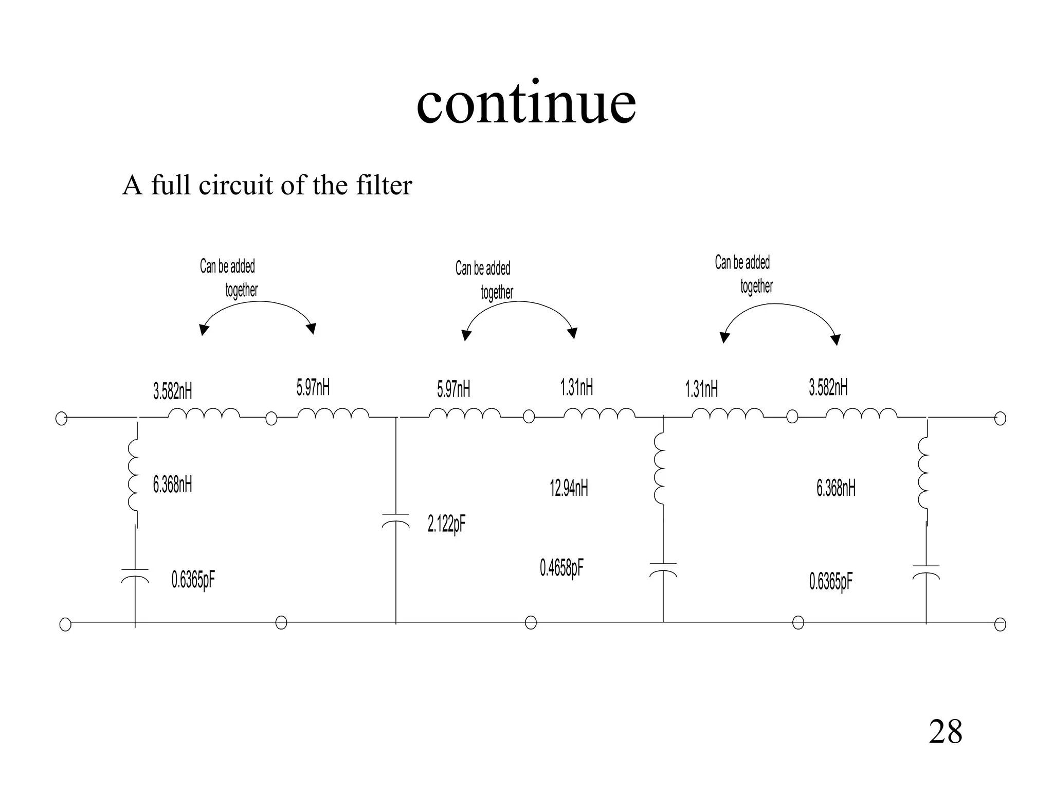
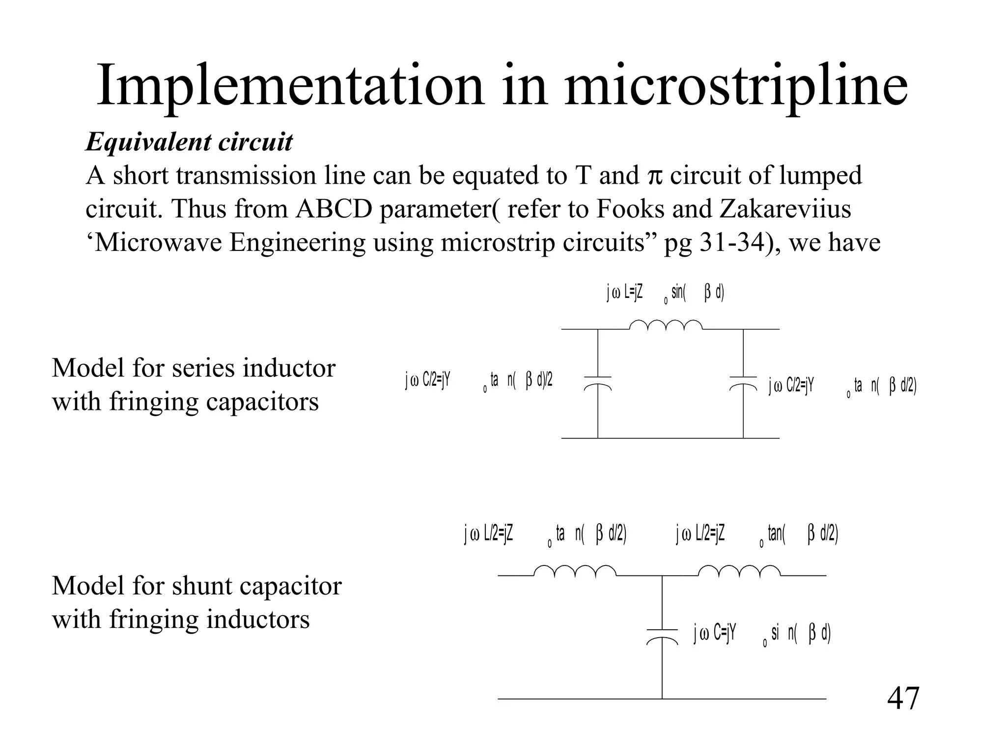
This document summarizes the design of microwave filters using composite, m-derived, T-network, and π-network sections. It describes: 1) How constant-k sections have very slow attenuation rates and non-constant image impedances. M-derived sections are introduced to address this by replacing component values to obtain the same image impedance as the constant-k section. 2) The propagation constant and image impedance equations for low-pass and high-pass T-network and π-network constant-k and m-derived sections. 3) Composite filters formed by combining m-derived and constant-k sections act as proper filters with rapid initial attenuation that does not reduce at higher


![FOURIER__ANALYSIS,[1].pptx](https://cdn.slidesharecdn.com/ss_thumbnails/fourieranalysis1-231113103452-b3aa5371-thumbnail.jpg?width=640&height=640&fit=bounds)


