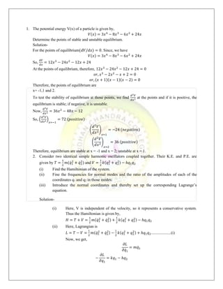
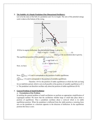
The document summarizes key concepts in classical dynamics related to small amplitude oscillations. It discusses: 1) Equilibrium and its types including static, dynamic, stable, unstable, and metastable equilibrium. 2) How potential energy minima correspond to points of stable equilibrium and small amplitude oscillations occur about these minima. 3) How the stability of a simple pendulum depends on the second derivative of its potential energy function. 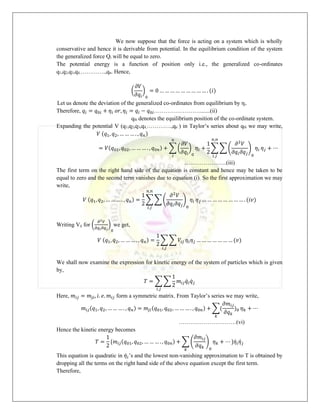4) The general problem of small oscillations is formulated by expanding the potential and kinetic energy functions as Taylor series about the equilibrium points and deriving the equations of motion. 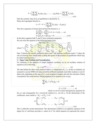5) The eigen value problem and normalization of the equations of motion allows representing the oscillations as a super

1. SEMESTER-VI
PHYSICS-DSE: CLASSICAL DYNAMICS
Small Amplitude Oscillations
The theory of small oscillations was developed by D’ Alembert, Joseph-Louis Lagrange and other
scientists. The study of the effect of all possible small perturbations to a dynamical system in mechanical
equilibrium is known as small oscillations. The theory of small oscillations is widely used in different
branches of physics viz. in acoustics, molecular spectra, coupled electric circuits etc.
1. Equilibrium and its types-
Equilibrium is the condition of a system in which all the forces- internal as well as external,
cancel out for some configuration of the system and unless the system is perturbed by an external
agency, it stays indefinitely in that state.
Equilibrium may be of following types-
a) Static Equilibrium-
Static equilibrium is a state of zero kinetic energy that continues indefinitely. In such
equilibrium the immediate surroundings of the system does not change with time. Example-
an object (e.g. book) lying still on a surface (e.g. table).
b) Dynamic Equilibrium-
Dynamic equilibrium is defined as the state when no net force acting on the system which
continues with zero kinetic energy. In such equilibrium the immediate surroundings of the
system change with time such that it exerts a balancing force on the system. Example- the
charge neutrality of atoms.
c) Stable Equilibrium-
In stable equilibrium, if a small displacement is given, the system tends to return to the
original equilibrium state. Example- the bob of a simple pendulum in equilibrium state.
d) Unstable Equilibrium-
In instable equilibrium, if a small displacement is given, the system does not return to the
original equilibrium state. Example- a large sized stone lying on the upper edge of a cliff.
e) Metastable Equilibrium-
In metastable equilibrium, the system can’t return to the original equilibrium configuration, if
displaced sufficiently; for smaller displacement, however, it can return. Example- a balloon
that explodes above a certain gas pressure.
2. Equilibrium state and stability of a system-
Small Amplitude Oscillations: Minima of potential energy and points of stable equilibrium, expansion
of the potential energy around minimum, small amplitude oscillations about the minimum, normal
modes of oscillations example of N identical masses connected in a linear fashion to (N -1) - identical
springs.

2. In a conservative system the potential V is a function of position (qi) only and the system is said
to be equilibrium when the generalized forces Qi acting on the system vanish.
Therefore, 𝑄𝑖 = − (
𝜕𝑉
𝜕𝑞𝑖
)
0
= 0 ………………………… (i)
i.e. the potential energy has an extremum (
maximum or minimum) at the equilibrium configuration of the system,
𝑞01, 𝑞02, 𝑞03, 𝑞04, … … … … … . , 𝑞0𝑛 . When V is a minimum at equilibrium, any small deviation
from this position means an increase in V and consequently decrease in kinetic energy T i.e.,
velocity v, in a conservative system and the body ultimately comes to rest, indicating the small
bounded motion about the Vmin. Such equilibrium is known as the stable equilibrium. On the
other hand, a small departure from Vmax results in decrease in V and increase in kinetic energy
and velocity indefinitely, which corresponds to unstable motion. Thus the position of Vmax is the
position of unstable equilibrium. Therefore oscillations always occur about a position of stable
equilibrium i.e. about Vmin.
Let V(max) be the potential energy function for a particle and also let
the force F acting on the particle vanishes at x0 i.e.
𝐹 = − (
𝑑𝑉
𝑑𝑥
)
𝑥0
= 0………………………….. (ii)
In that case x0 is the point of equilibrium. To test the stability of the equilibrium we must examine
𝑑2𝑉
𝑑𝑥2 at x0. If the second derivative is positive, the equilibrium is stable. Thus in stable
equilibrium,
(
𝑑2
𝑉
𝑑𝑥2
)𝑥0
> 0
If the second derivative is negative, the equilibrium is unstable. Thus in unstable equilibrium,
(
𝑑2
𝑉
𝑑𝑥2
)𝑥0
< 0
And if the second derivative also vanishes, we must examine the higher derivatives at x0. If all the
derivatives vanish at x0, so that V(x) is constant in a region about x0, then the particle is
effectively free. In such a situation no force results from a displacement (from x0 ) and the system
to be in state of neutral stability. Thus in neutral equilibrium,
(
𝑑2
𝑉
𝑑𝑥2
)𝑥0
= 0

3. 3. The Stability of a Simple Pendulum (One Dimensional Oscillator)-
Let m be the mass of the bob of a pendulum and l be its length. The zero of the potential energy
scale is taken at the bottom of the swing.
If Ө be its angular deflection, then the potential energy is given by,
𝑉(𝜃) = 𝑚𝑔𝑙(1 − 𝐶𝑜𝑠𝜃)……………………….. (i)
where g is the acceleration due to gravity.
The equilibrium position of the pendulum is given by,
𝑑𝑉
𝑑𝜃
= 𝑚𝑔𝑙 𝑆𝑖𝑛𝜃 = 0
𝑖. 𝑒. Ө = 𝑒𝑖𝑡ℎ𝑒𝑟 0 𝑜𝑟 𝜋
Now, we have
𝑑2
𝑉
𝑑𝜃2
= 𝑚𝑔𝑙 𝐶𝑜𝑠𝜃
Now, (
𝑑2𝑉
𝑑𝜃2)𝜃=0 > 0, and it corresponds to the position of stable equilibrium.
(
𝑑2𝑉
𝑑𝜃2)𝜃=𝜋 < 0, and it corresponds to the position of unstable equilibrium.
Therefore Ө=0 is the position of stable equilibrium at which the bob can hang
for an indefinite period, which is not at all possible at the position of unstable equilibrium at 𝜃 =
𝜋. The pendulum can therefore oscillate only about the position of stable equilibrium (Ө=0).
4. General Problem of Small Oscillation-
a) Formulation of the Problem-
In tackling the general problem of small oscillations we perform an appropriate simplification of
Lagrangian method. We know that the oscillations whether large or small take place about a
position of equilibrium. Thus a pendulum oscillates about a verticval which is its stable
equilibrium position. When the pendulum is deflected from the stable position a restoring force
acts on the pendulum in a direction opposite to the direction of deflection. In the equilibrium
position this force is zero.

4. We now suppose that the force is acting on a system which is wholly
conservative and hence it is derivable from potential. In the equilibrium condition of the system
the generalized force Qi will be equal to zero.
The potential energy is a function of position only i.e., the generalized co-ordinates
q1,q2,q3,q4,………….,qn. Hence,
(
𝜕𝑉
𝜕𝑞𝑖
)
0
= 0 … … … … … … … … … . (𝑖)
Let us denote the deviation of the generalized co-ordinates from equilibrium by ηi.
Therefore, 𝑞𝑖 = 𝑞0𝑖 + 𝜂𝑖 𝑜𝑟, 𝜂𝑖 = 𝑞𝑖 − 𝑞0𝑖…………………….......(ii)
q0i denotes the equilibrium position of the co-ordinate system.
Expanding the potential V (q1,q2,q3,q4,………….,qn ) in Taylor’s series about q0i we may write,
𝑉 (𝑞1, 𝑞2, … … … . , 𝑞𝑛)
= 𝑉(𝑞01, 𝑞02, … … … . , 𝑞0𝑛) + ∑ (
𝜕𝑉
𝜕𝑞𝑖
)
0
𝑛
𝑖
𝜂𝑖 +
1
2
∑ ∑ (
𝜕2
𝑉
𝜕𝑞𝑖𝜕𝑞𝑗
)
0
𝜂𝑖
𝑛,𝑛
𝑖,𝑗
𝜂𝑗 + ⋯
………………….(iii)
The first term on the right hand side of the equation is constant and hence may be taken to be
equal to zero and the second term vanishes due to equation (i). So the first approximation we may
write,
𝑉 (𝑞1, 𝑞2, … … … . , 𝑞𝑛) =
1
2
∑ ∑ (
𝜕2
𝑉
𝜕𝑞𝑖𝜕𝑞𝑗
)
0
𝜂𝑖
𝑛,𝑛
𝑖,𝑗
𝜂𝑗 … … … … … … … … . (𝑖𝑣)
Writing Vij for (
𝜕2𝑉
𝜕𝑞𝑖𝜕𝑞𝑗
)
0
we get,
𝑉 (𝑞1, 𝑞2, … … … . , 𝑞𝑛) =
1
2
∑ ∑ 𝑉𝑖𝑗
𝑖,𝑗
𝜂𝑖𝜂𝑗 … … … … … … … (𝑣)
We shall now examine the expression for kinetic energy of the system of particles which is given
by,
𝑇 = ∑ ∑
1
2
𝑚𝑖𝑗𝑞̇𝑖𝑞̇𝑗
𝑖,𝑗
Here, 𝑚𝑖𝑗 = 𝑚𝑗𝑖, 𝑖. 𝑒. 𝑚𝑖𝑗 form a symmetric matrix. From Taylor’s series we may write,
𝑚𝑖𝑗(𝑞1, 𝑞2, … … … . , 𝑞𝑛) = 𝑚𝑗𝑖(𝑞01, 𝑞02, … … … . , 𝑞0𝑛) + ∑(
𝜕𝑚𝑖𝑗
𝜕𝑞𝑘
)0
𝑘
𝜂𝑘 + ⋯
…………………………(vi)
Hence the kinetic energy becomes
𝑇 =
1
2
{𝑚𝑖𝑗(𝑞01, 𝑞02, … … … . , 𝑞0𝑛) + ∑ (
𝜕𝑚𝑖𝑗
𝜕𝑞𝑘
)
0
𝑘
𝜂𝑘 + ⋯ }𝜂̇𝑖𝜂̇𝑗
This equation is quadratic in 𝜂̇𝑖’s and the lowest non-vanishing approximation to T is obtained by
dropping all the terms on the right hand side of the above equation except the first term.
Therefore,

5. 𝑇 =
1
2
∑ ∑ 𝑚𝑖𝑗(𝑞01, 𝑞02, … … … . , 𝑞0𝑛)𝜂̇𝑖𝜂̇𝑗 =
1
2
∑ ∑ 𝑇𝑖𝑗 𝜂̇𝑖𝜂̇𝑗
………………………………..(vii)
Here the constant value of mij at equilibrium is denoted by Tij.
Hence the Lagrangian function is,
𝐿 = 𝑇 − 𝑉 =
1
2
∑ ∑(𝑇𝑖𝑗
𝑖,𝑗
𝜂̇𝑖𝜂̇𝑗 − 𝑉𝑖𝑗𝜂𝑖𝜂𝑗)
Thus the n-equations of motion derived from the function L is
𝑑
𝑑𝑡
(
𝜕𝐿
𝜕𝜂̇𝑖
) − (
𝜕𝐿
𝜕𝜂𝑖
) = 0 (𝑖 = 1,2,3, … . . , 𝑛)
𝑜𝑟, ∑ 𝑇𝑖𝑗 𝜂̈𝑗 + ∑ 𝑉𝑖𝑗𝜂𝑗 = 0…………………..(viii)
In the above equation both Tij and Vij have symmetric properties.
We can write this equation in the following matrix form,
𝑇𝜂̈ + 𝑉𝜂 = 0……………...............……..(ix)
where 𝑇 = (
𝑇11 𝑇12 … 𝑇1𝑛
𝑇21 𝑇22 … 𝑇2𝑛
… … … …
𝑇𝑛1 𝑇𝑛2 … 𝑇𝑛𝑛
) ; 𝑉 = (
𝑉11 𝑉12 … 𝑉1𝑛
𝑉21 𝑉22 … 𝑉2𝑛
… … … …
𝑉𝑛1 𝑉𝑛2 … 𝑉
𝑛𝑛
) ; 𝜂 = (
𝜂1
𝜂2
⋮
𝜂𝑛
)
Here T denotes the inertial coefficient matrix and V the stiffness coefficient matrix. V plays the
role of restoring force which tends to bring the system to the position of equilibrium which may
be called restoring tensor.
b) Eigen Value Problem and Normalization-
For similarity to the equation of simple harmonic oscillator, we try an oscillator solution of
equation (viii) in the form,
𝜂𝑗 = 𝑎𝑗𝑒𝑖𝜔𝑡
…………………………………….(x)
The idea behind the above trial solution is that ω is independent of j, i.e. all the co-ordinates are
assumed to execute SHM with same period but different amplitude (and either in-phase or out-of-
phase only, depending on the sign of aj ). aj are in general complex and only the real parts of them
correspond to the actual motion. Putting equation (x) in equation (viii) we get,
∑(𝑉𝑖𝑗 − 𝜔2
𝑇𝑖𝑗)𝑎𝑗 = 0
𝑗
…………………..(xi)
(𝑖 = 1,2,3, … … … … … , 𝑛)
which is a set of n linear homogeneous equations for
the aj’s and consequently for a non-trivial solution (i.e., not all aj =0) the determinant of the
coefficients must vanish i.e. ⎹𝑉𝑖𝑗 − 𝜔2
𝑇𝑖𝑗⎹ = 0
𝑜𝑟, |
𝑉11 − 𝜔2
𝑇11 … … 𝑉1𝑛 − 𝜔2
𝑇1𝑛
⋮ ⋮
⋮ ⋮
𝑉𝑛1 − 𝜔2
𝑇𝑛1 … … 𝑉
𝑛𝑛 − 𝜔2
𝑇𝑛𝑛
| = 0
....................................... (xii)
This is called the secular determinant. This determinant condition is an algebraic equation of nth
degree for 𝜔2
and hence provides n- values of 𝜔2
for which equation (x) represents the correct

6. solutions to the equations of motion. For each of these values of 𝜔2
the equation (xi) may be
solved for the amplitudes or more precisely for (n-1) of the amplitudes in terms of the remaining
one. This is due to the fact that the coefficient aj are determined only up to a common multiplier.
This is apparent from equation (xi). Thus the ratios of aj’s are definite (for a particular frequency)
but not their absolute values. This arbitrariness in the values of aj will be utilized in the
normalization procedure.
Since there exist n values of 𝜔𝑘, we also get n- set of values of
amplitudes. Each of these set (i.e., n- values of aj’s corresponding to a particular frequency(𝜔𝑘)
can be considered to define the components of a n- dimensional vector 𝑎
⃗𝑘. This 𝑎
⃗𝑘 is called the
eigen vector of the system associated with the eigen frequency𝜔𝑘. The symbol ajk may now be
used to represent the j-th component of the k-th eigen vector. Using the principle of
superposition, the general solution may now be written as,
𝜂𝑗(𝑡) = ∑ 𝑎𝑗𝑘𝑒𝑖𝜔𝑘𝑡
𝑘
....................................... (xiii)
where motion of each ηj is compounded of motions with each of the n values of frequencies 𝜔𝑘.
The actual motion is the real part of the complex equation (xiii) which can be expressed as,
𝜂𝑗(𝑡) = ∑ 𝑎𝑗𝑘 𝐶𝑜𝑠(
𝑘
𝜔𝑘𝑡 + 𝜙𝑘)
The motion is oscillatory about the stable equilibrium position only for 𝜔𝑘
2
> 0. If two or more
values of 𝜔𝑘 happen to be the same, then the phenomenon is known as degeneracy.
c) Orthogonality of Eigenvectors-
Equation (xi) represents a special type of eigen value equation as,
𝑽𝒂 = 𝝀𝑻𝒂 ..........................................(xiv) with 𝜔2
= 𝜆
where the matrix V,T and a are
𝑽 = (
𝑉11 𝑉12 … 𝑉1𝑛
𝑉21 𝑉22 … 𝑉2𝑛
… … … …
𝑉𝑛1 𝑉𝑛2 … 𝑉
𝑛𝑛
), 𝑻 = (
𝑇11 𝑇12 … 𝑇1𝑛
𝑇21 𝑇22 … 𝑇2𝑛
… … … …
𝑇𝑛1 𝑇𝑛2 … 𝑇𝑛𝑛
), 𝒂 = (
𝑎1
𝑎2
⋮
𝑎𝑛
)
In ordinary eigenvalue problem, 𝑽𝒂 = 𝜆𝒂 i.e. the effect of V on eigenvector a is just to generate a
vector which is 𝜆 times a, 𝜆 being a scalar. Here, however, V acting on a, generates a multiple (𝜆)
of the result of T acting on a.
A typical equation for the eigenvalue 𝜆𝑘 can be written from equation (xiv) as,
∑ 𝑉𝑖𝑗𝑎𝑗𝑘 = 𝜆𝑘 ∑ 𝑇𝑖𝑗𝑎𝑗𝑘
𝑗
𝑗
......................................(xv)
The complex conjugate of similar equation for λl gives,
∑ 𝑉𝑖𝑗𝑎𝑖𝑙
∗
= 𝜆𝑙
∗
∑ 𝑇𝑖𝑗
𝑗
𝑗
𝑎𝑖𝑙
∗
.........................................(xvi)
(since Vij and Tij are real and also symmetric)
Multiplying equation (xv) by 𝑎𝑖𝑙
∗
and summing over i and multiplying equation (xvi) by ajk and
summing over j, and next subtracting the latter from the former, we get

7. (𝜆𝑘 − 𝜆𝑙
∗
) ∑ 𝑇𝑖𝑗𝑎𝑗𝑘
𝑖𝑗
𝑎𝑖𝑙
∗
= 0 … … … … … … … (𝑥𝑣𝑖𝑖)
𝑜𝑟, (𝜆𝑘 − 𝜆𝑘
∗
) ∑ 𝑇𝑖𝑗𝑎𝑗𝑘
𝑖𝑗
𝑎𝑖𝑘
∗
= 0
............................................(xviii) for l=k
Now, 𝑎𝑗𝑘 = 𝛼𝑗𝑘 + 𝑖𝛽𝑗𝑘 as ajk is complex.
and
∑ 𝑇𝑖𝑗𝑎𝑗𝑘𝑎𝑖𝑘
∗
= ∑ 𝑇𝑖𝑗𝛼𝑗𝑘
𝑖𝑗
𝛼𝑖𝑘 + ∑ 𝑇𝑖𝑗𝛽𝑗𝑘
𝑖𝑗
𝛽𝑖𝑘 + 𝑖 ∑ 𝑇𝑖𝑗(𝛽𝑗𝑘𝛼𝑖𝑘 − 𝛼𝑗𝑘𝛽𝑖𝑘) … … … … . . (𝑥𝑖𝑥)
Tij being symmetric, the interchange of dummy indices i and j changes sign
of the third summation on the right. Therefore, the imaginary term vanishes in equation (xix) and
the two real sums are twice the kinetic energy when the velocities 𝜂̇𝑖 have values 𝛼𝑖𝑘 and 𝛽𝑖𝑘
respectively. The kinetic energy can never be zero for real velocities. Thus, the eigenvalues 𝜆𝑘
must be real.
Eigenvalues and eigenvectors being real, the equation (xvii) may be written as
(𝜆𝑘 − 𝜆𝑙) ∑ 𝑇𝑖𝑗𝑎𝑗𝑘
𝑖𝑗
𝑎𝑖𝑙 = 0 … … … … … … … … … . (𝑥𝑥)
When the roots of the characteristic equation (xii) are all distinct, 𝜆𝑘 ≠ 𝜆𝑙, we shall get,
∑ 𝑇𝑖𝑗𝑎𝑗𝑘 𝑎𝑖𝑙 = 0 … … … … … … … … … … … … (𝑥𝑥𝑖)(𝑓𝑜𝑟 𝑙 ≠ 𝑘)
This shows that the eigenvectors are orthogonal.
The eigenvalue equation (xi) can’t completely fix the values of ajk, as has already been stated. The
uncertainty can however be removed be removed by setting, purely arbitrarily,
∑ 𝑇𝑖𝑗𝑎𝑗𝑘
𝑖𝑗
𝑎𝑖𝑘 = 1 … … … … … … … … … … … (𝑥𝑥𝑖𝑖)(𝑓𝑜𝑟 𝑙 = 𝑘)
Each of n such equations uniquely fix the arbitrary component in each eigenvector
(corresponding to a given eigenfrequency). Combining the equations (xxi) and (xxii), we get
∑ 𝑇𝑖𝑗𝑎𝑗𝑘
𝑖𝑗
𝑎𝑖𝑘 = 𝛿𝑙𝑘
𝑖. 𝑒. 𝒂
̃𝑻𝒂 = 𝑰................................(xxiii)
where 𝒂
̃ being the transpose of a.
Introducing a diagonal matrix λ with elements 𝜆𝑙𝑘 = 𝜆𝑘𝛿𝑙𝑘, the eigenvalue equation (xv) becomes
∑ 𝑉𝑖𝑗𝑎𝑗𝑘 = 𝜆𝑘 ∑ 𝑇𝑖𝑗𝑎𝑗𝑘
𝑗
𝑗
= ∑ 𝑇𝑖𝑗
𝑗𝑖
𝑎𝑗𝑙𝜆𝑙𝑘
𝑖. 𝑒. 𝑽𝒂 = 𝑻𝒂𝜆 … … … … … … … . . (𝑥𝑥𝑖𝑣)
Therefore, 𝒂
̃𝑽𝒂 = 𝒂
̃𝑻𝒂𝜆 = 𝜆..........................(xxv)
This shows that the matrix a diagonalises both T and V simultaneously.
d) Normal co-ordinates-
The normalization of ajk leaves no ambiguity in the solution for 𝜂𝑗. To remove the loss of
generality due to the introduction of arbitrary normalization, a scalar factor βk may be used when
the equation (xiii) becomes

8. 𝜂𝑗(𝑡) = ∑ 𝑎𝑗𝑘𝛽𝑘𝑒𝑖𝜔𝑘𝑡
= ∑ 𝑎𝑗𝑘𝑄𝑘 … … … … … … … … (𝑥𝑥𝑣𝑖)
𝑘
𝑘
where 𝑄𝑘 = 𝛽𝑘𝑒𝑖𝜔𝑘𝑡
............................(xxvii)
Therefore, 𝜼
̃ = 𝒂
̃𝑸
̃..........................(xxviii)
Equation (xxvii) shows that Qk oscillates with one frequency only, called normal frequency,
namely 𝜔𝑘. These Qk’s are called the normal co-ordinates of the system. The normal co-ordinates
are thus defined as the generalized co-ordinates where each one of them executes oscillations
with a single frequency. If expressed in terms of normal co-ordinates, potential energy and kinetic
energy take rather simple forms as given below,
𝑃. 𝐸. = 𝑉 =
1
2
∑ 𝜂𝑖𝑉𝑖𝑗𝜂𝑗 =
1
2
𝑖𝑗
𝜼
̃𝑽𝜼 =
1
2
𝑄
̃𝒂
̃𝑽𝒂𝑄 =
1
2
𝑄
̃𝜆𝑄
=
1
2
∑ 𝑄𝑙𝜆𝑙𝑘𝑄𝑘
𝑙𝑘
=
1
2
∑ 𝑄𝑙𝜆𝑘𝛿𝑙𝑘𝑄𝑘 =
𝑙𝑘
1
2
∑ 𝜔𝑘
2
𝑄𝑘
2
𝑘
… … … … . . (𝑥𝑥𝑖𝑥)
(using equations (xxviii) and (xxv))
𝐾. 𝐸 = 𝑇 =
1
2
∑ 𝜂̇𝑖𝑇𝑖𝑗
𝑖𝑗
𝜂̇𝑗 =
1
2
𝜂̇
̃𝑇𝜂̇ =
1
2
𝑄̇
̃𝒂
̃𝑻𝒂𝑄̇ =
1
2
𝑄̇
̃𝑄̇ =
1
2
∑ 𝑄̇𝑘
2
… … … … … … . (𝑥𝑥𝑥)
𝑘
So, the new Lagrangian is,
𝐿 = 𝑇 − 𝑉 =
1
2
∑(𝑄̇𝑘
2
−
𝑘
𝜔𝑘
2
𝑄𝑘
2
) … … … … … … … … . . (𝑥𝑥𝑥𝑖)
Therefore, the Lagrange’s equation of motion are given by,
𝑑
𝑑𝑡
(
𝜕𝐿
𝜕𝑄̇𝑘
) −
𝜕𝐿
𝜕𝑄
= 0
𝑜𝑟, 𝑄̈𝑘 + 𝜔𝑘
2
𝑄𝑘 = 0 … … … … … … … … … … … (𝑥𝑥𝑥𝑖𝑖) (k=1,2,3......)
This is the set of n-independent equations of SHM with single normal frequency 𝜔𝑘.
The solution of the equation (xxxii) is given by,
𝑄𝑘 = 𝑎𝑘𝐶𝑜𝑠(𝜔𝑘𝑡) + 𝑏𝑘𝑆𝑖𝑛(𝜔𝑘𝑡), 𝑤ℎ𝑒𝑛 𝜔𝑘
2
> 0
𝑄𝑘 = 𝑎𝑘𝑡 + 𝑏𝑘𝑡, 𝑤ℎ𝑒𝑛 𝜔𝑘
2
= 0
𝑄𝑘 = 𝑎𝑘𝑒𝜔𝑘𝑡
+ 𝑏𝑘𝑒−𝜔𝑘𝑡
, 𝑤ℎ𝑒𝑛 𝜔𝑘
2
< 0
For 𝜔𝑘
2
> 0, the co-ordinates always remain finite. Such solutions refer to stable
equilibrium. For 𝜔𝑘
2
= 0 and 𝜔𝑘
2
< 0, the co-ordinates become infinite as time advances and
such solutions refer to unstable equilibrium.
e) Normal co-ordinates Qk in terms of co-ordinates ηj
The complex quantity βk may be written as,

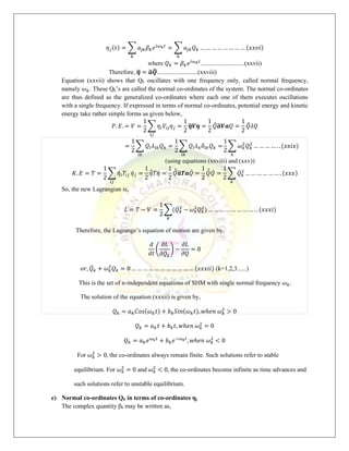
9. 𝛽𝑘 = 𝜇𝑘 + 𝑖𝜈𝑘.................................................(xxxiii)
Therefore, equation (x) becomes,
𝜂𝑗(𝑡) = ∑ 𝑎𝑗𝑘(
𝑘
𝜇𝑘 + 𝑖𝜈𝑘)𝑒𝑖𝜔𝑘𝑡
............................(xxxiv)
On differentiating with respect to time we get,
𝜂
̇ 𝑗(𝑡) = ∑ 𝑖𝜔𝑘𝑎𝑗𝑘(
𝑘
𝜇𝑘 + 𝑖𝜈𝑘)𝑒𝑖𝜔𝑘𝑡
................................................(xxxv)
The real part of equation (xxxiv) gives at t=0,
𝜂𝑗(0) = ∑ 𝑎𝑗𝑘
𝑘
𝜇𝑘
............................................(xxxvi)
Multiplying throughout by Tjiair and summing over ij, and using equation (xxxvi), we get,
∑ 𝜂𝑗(0)𝑇𝑗𝑖𝑎𝑖𝑟 = ∑ 𝜇𝑘
𝑘
∑ 𝑎𝑗𝑘
𝑖𝑗
𝑖𝑗
𝑇𝑗𝑖𝑎𝑖𝑟 = ∑ 𝜇𝑘𝛿𝑘𝑟 = 𝜇𝑟
𝑘
..........................(xxxvii)
Similarly, the real part of equation (xxxv) at t=0 gives,
𝜂̇𝑗(0) = − ∑ 𝜔𝑘
𝑘
𝜈𝑘𝑎𝑗𝑘
...................................(xxxviii)
Multiplying both sides by Tjiair and summing over ij, and using equation(xxxvi), we get,
∑ 𝜂̇𝑗(0)𝑇𝑗𝑖𝑎𝑖𝑟 = − ∑ 𝜔𝑘𝜈𝑘
𝑘
∑ 𝑎𝑗𝑘
𝑖𝑗
𝑖𝑗
𝑇𝑗𝑖𝑎𝑖𝑟 = − ∑ 𝜔𝑘𝜈𝑘𝛿𝑘𝑟 = −𝜔𝑟
𝑘
𝜈𝑟
.......................(xxxix)
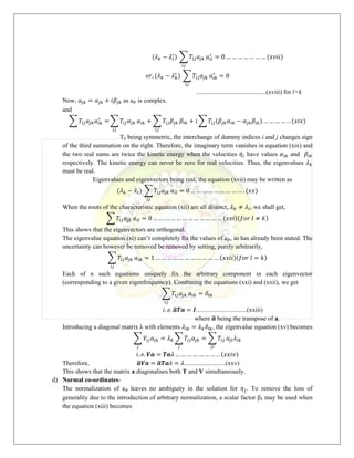
Thus, the normal co-ordinates Qr may be expressed as the real part of the expression in,
𝑄𝑟(𝑡) = 𝛽𝑟𝑒𝑖𝜔𝑟𝑡
= (𝜇𝑟 + 𝑖𝜈𝑟)𝑒𝑖𝜔𝑟𝑡
= ∑ 𝑇𝑗𝑖𝑎𝑖𝑟[
𝑖𝑗
𝜂𝑗(0) −
𝑖
𝜔𝑟
𝜂̇𝑗(0)]𝑒𝑖𝜔𝑟𝑡
Therefore, for any arbitrary 𝜂𝑗(0) and 𝜂̇𝑗(0), a set of normal co-ordinates Qr may be found, each
of which varies harmonically with single frequency 𝜔𝑟.
f) Energy in normal co-ordinates
Here,
𝑉 =
1
2
∑ 𝜔𝑘
2
𝑄𝑘
2
𝑘 and 𝑇 =
1
2
∑ 𝑄̇𝑘
2
𝑘
So, total mechanical energy E, in normal co-ordinates, is given by,
𝐸 = 𝑇 + 𝑉 =
1
2
∑(𝑄̇𝑘
2
+ 𝜔𝑘
2
𝑄𝑘
2
)
𝑘
This is true for small oscillations with any number n of degrees of freedom.
Examples-

10. 1. The potential energy V(x) of a particle is given by,
𝑉(𝑥) = 3𝑥4
− 8𝑥3
− 6𝑥2
+ 24𝑥
Determine the points of stable and unstable equilibrium.
Solution-
For the points of equilibrium(𝑑𝑉/𝑑𝑥) = 0. Since, we have
𝑉(𝑥) = 3𝑥4
− 8𝑥3
− 6𝑥2
+ 24𝑥
So,
𝑑𝑉
𝑑𝑥
= 12𝑥3
− 24𝑥2
− 12𝑥 + 24
At the points of equilibrium, therefore, 12𝑥3
− 24𝑥2
− 12𝑥 + 24 = 0
𝑜𝑟, 𝑥3
− 2𝑥2
− 𝑥 + 2 = 0
𝑜𝑟, (𝑥 + 1)(𝑥 − 1)(𝑥 − 2) = 0
Therefore, the points of equilibrium are
x= -1,1 and 2.
To test the stability of equilibrium at those points, we find
𝑑2𝑉
𝑑𝑥2 at the points and if it is positive, the
equilibrium is stable; if negative, it is unstable.
Now,
𝑑2𝑉
𝑑𝑥2 = 36𝑥2
− 48𝑥 − 12
So, (
𝑑2𝑉
𝑑𝑥2)
𝑥=−1
= 72 (𝑝𝑜𝑠𝑖𝑡𝑖𝑣𝑒)
(
𝑑2
𝑉
𝑑𝑥2)
𝑥=1
= −24 (𝑛𝑒𝑔𝑎𝑡𝑖𝑣𝑒)
(
𝑑2
𝑉
𝑑𝑥2)
𝑥=2
= 36 (𝑝𝑜𝑠𝑖𝑡𝑖𝑣𝑒)
Therefore, equilibrium are stable at x = -1 and x = 2; unstable at x = 1.
2. Consider two identical simple harmonic oscillators coupled together. Their K.E. and P.E. are
given by 𝑇 =
1
2
𝑚(𝑞̇1
2
+ 𝑞̇2
2
) and 𝑉 =
1
2
𝑘(𝑞1
2
+ 𝑞2
2) − ℎ𝑞1𝑞2
(i) Find the Hamiltonian of the system.
(ii) Fine the frequencies for normal modes and the ratio of the amplitudes of each of the
coordinates q1 and q2 in those modes.
(iii) Introduce the normal coordinates and thereby set up the corresponding Lagrange’s
equation.
Solution-
(i) Here, V is independent of the velocity, so it represents a conservative system.
Thus the Hamiltonian is given by,
𝐻 = 𝑇 + 𝑉 =
1
2
𝑚(𝑞̇1
2
+ 𝑞̇2
2) +
1
2
𝑘(𝑞1
2
+ 𝑞2
2) − ℎ𝑞1𝑞2
(ii) Here, Lagrangian is
𝐿 = 𝑇 − 𝑉 =
1
2
𝑚(𝑞̇1
2
+ 𝑞̇2
2) −
1
2
𝑘(𝑞1
2
+ 𝑞2
2) + ℎ𝑞1𝑞2....................(i)
Now, we get,
𝜕𝐿
𝜕𝑞̇1
= 𝑚𝑞̇1
−
𝜕𝐿
𝜕𝑞1
= 𝑘𝑞1 − ℎ𝑞2

11. 𝜕𝐿
𝜕𝑞̇2
= 𝑚𝑞̇2
−
𝜕𝐿
𝜕𝑞2
= 𝑘𝑞2 − ℎ𝑞1
Putting these values in equation (i) we get,
𝑚𝑞̈1 + 𝑘𝑞1 − ℎ𝑞2 = 0...................(ii)
𝑚𝑞̈2 + 𝑘𝑞1 − ℎ𝑞2 = 0...................(iii)
Let 𝑞1 = 𝐴1𝑒𝑖𝜔𝑡
. Putting this value in equation (ii) we get,
𝐴1(𝑘 − 𝜔2
𝑚) − 𝐴2ℎ = 0
Again, let 𝑞2 = 𝐴2𝑒𝑖𝜔𝑡
. Putting this value in equation (iii) we get,
−𝐴1ℎ + 𝐴2(𝑘 − 𝜔2
𝑚) = 0
For non-zero solution, we must have the determinant,
|𝑘 − 𝜔2
𝑚 −ℎ
−ℎ 𝑘 − 𝜔2
𝑚
| = 0
𝑜𝑟, (𝑘 − 𝜔2
𝑚)2
− ℎ2
= 0
𝑜𝑟, 𝑘 − 𝜔2
𝑚 = ±ℎ
Therefore, 𝜔2
= (𝑘 ∓ ℎ)
So, 𝜔1 = √
(𝑘−ℎ)
𝑚
, 𝜔2 = √
(𝑘+ℎ)
𝑚
Now,
𝐴2
𝐴1
=
(𝑘−𝜔1
2
𝑚)
ℎ
𝑜𝑟,
(𝑘−𝜔2
2
𝑚)
ℎ
(iii) Let the normal coordinates are 𝑄𝑖 = 𝐴𝑖𝑒𝑖𝜔𝑖𝑡
Differentiating with respect to t we get,
𝑄̈𝑖 + 𝜔𝑖
2
𝑄𝑖 = 0, 𝑖 = 1,2.
Thus Lagrange’s equation is,
𝐿𝑖 =
1
2
𝑄̇𝑖
2
−
1
2
𝜔𝑖𝑄𝑖
2
Exercise-
1. The potential energy of a particle is given by
𝑉(𝑥) = 𝑥4
− 4𝑥3
− 8𝑥2
+ 48𝑥
Find the points of stable and unstable equilibrium. (KNU-2019)
2. Discuss the general theory of small oscillation of a system to obtain the equation of motion near
its equilibrium position. How the eigen frequencies of the system can be obtained for such a
system. (KNU-2019)
3. What is normal mode and normal frequency? (KNU-2019)
4. Discuss the stability of a simple pendulum and show that it can oscillate only about the position
of its stable equilibrium.
5. Establish the relation
𝑇𝜂̈ + 𝑉𝜂 = 0,for small oscillations of a system, the symbols
having their usual meanings.
6. A particle moves in potential energy given by

12. 𝑉(𝑥) = 𝑏𝑥2
+
𝑎
𝑥2, a,b>0. Show that its frequency of oscillation is √
8𝑏
𝑚
.
7. What is meant by equilibrium, stable and unstable equilibrium? Show that oscillations can occur
only about a stable equilibrium.
8. Write down the differences between stable and unstable equilibrium.
References-
1) S.N.Maithi & D.P.Raychaudhuri, Classical Mechanics and General Properties of Matter, New Age International Publishers,
2015
2) A.B.Gupta, Fundamentals of Classical Mechanics, 2nd
Edition, Books And Allied (P) Ltd. (2019)
3) A. Beiser, Perspective of Modern Physics, 3rd
Edition, New York, McGraw Hill (1969).
AJAY KUMAR SHARMA
Assistant Professor (Physics)
B.C.College, Asansol
Email-id- ajay888sharma@yahoo.co.in