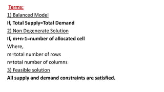
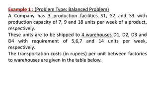
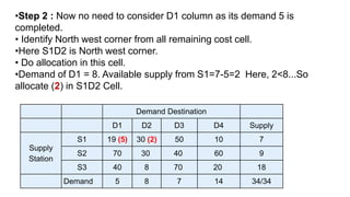
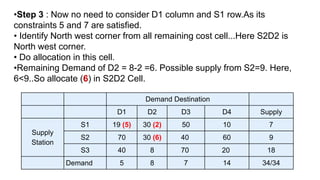
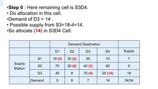
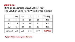
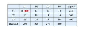
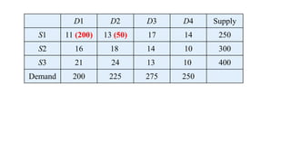
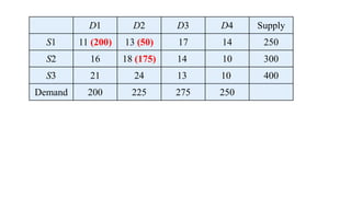
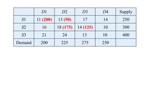
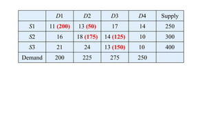
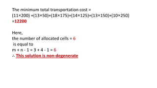
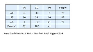
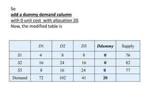
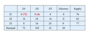
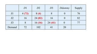
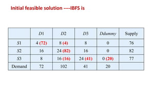
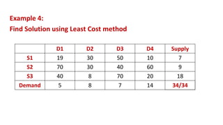
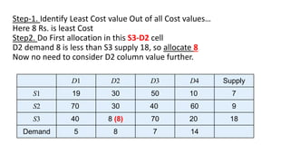
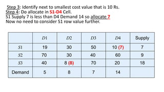
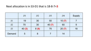
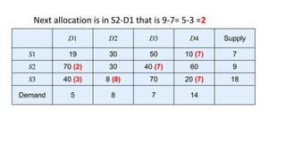
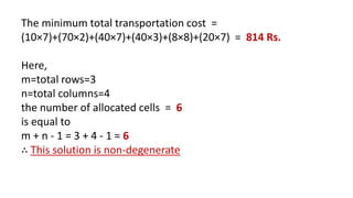
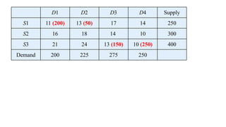
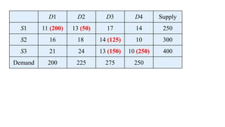
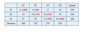
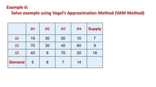
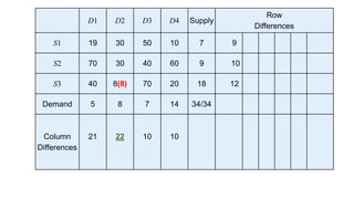
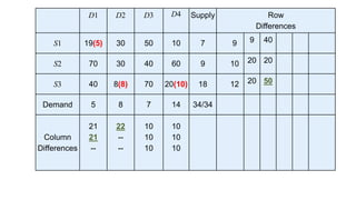
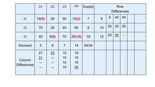
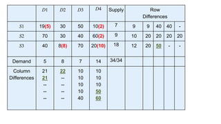
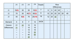
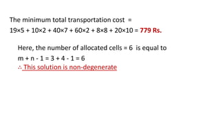
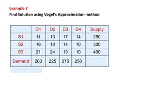
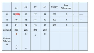
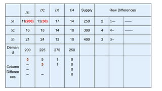
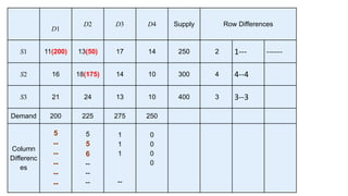
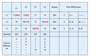
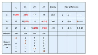
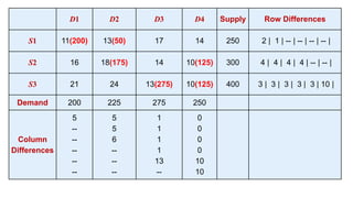
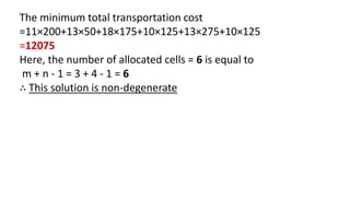
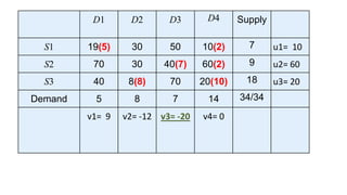
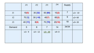
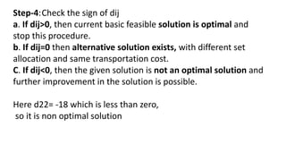
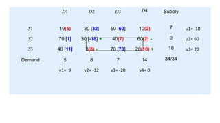
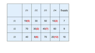
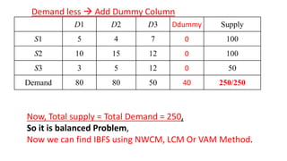
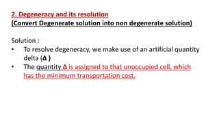
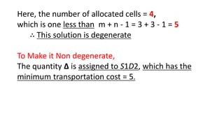
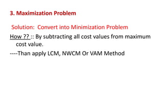
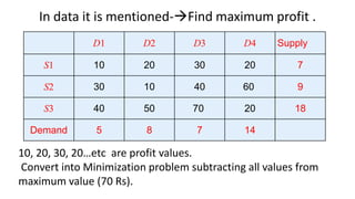
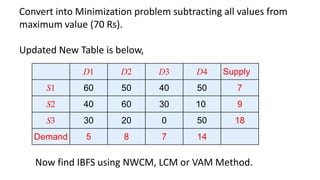
Transportation Method Initial Basic Feasible Solution-IBFS North West Corner Method--NWCM , Least Cost Method--LCM and Vogel’s Approximation Method--VAM Optimality Test using Modified Distribution Method-MODI method. Variation in transportation Unbalance Supply and Demand Degeneracy and its resolution Maximization Problem

1. Operations Research
Chapter : Transportation
Find Initial Basic Feasible Solution-IBFS Using
North West Corner Method-- NWCM ,
Least Cost Method-- LCM and
Vogel’s Approximation Method-- VAM
Optimality Test using Modified Distribution Method-
MODI method.
Variation in transportation
Unbalance Supply and Demand
Degeneracy and its resolution
Maximization Problem

2. Introduction
• Transportation Models are used to find out optimum cost of
transportation of goods.
• Company ABC has three plants at Ahmedabad, Surat and Rajkot and
four demand stations at Visnagar, Baroda and Vapi and Bhuj. We
can formulate transportation matrix as below
Visnagar Baroda Vapi Bhuj Capacity
Ahmedabad 10 20 30 40 7
Surat 20 30 10 60 8
Rajkot 20 15 40 20 5
Demand 2 7 6 5 20

3. Here,
In table cell value 10,20,30,40 Rs. shows cost of transportation.
Last column value shows daily maximum supply.
Last row value shows daily maximum demand of each city.

4. Terms:
1) Balanced Model
If, Total Supply=Total Demand
2) Non Degenerate Solution
If, m+n-1=number of allocated cell
Where,
m=total number of rows
n=total number of columns
3) Feasible solution
All supply and demand constraints are satisfied.

5. Methods to find out Initial Basic Feasible Solution (IBFS):
1. NWCM-- North West Corner Method
2. LCM-- Least Cost Method
3. VAM-- Vogel’s Approximation Method

6. Example 1 : (Problem Type: Balanced Problem)
A Company has 3 production facilities S1, S2 and S3 with
production capacity of 7, 9 and 18 units per week of a product,
respectively.
These units are to be shipped to 4 warehouses D1, D2, D3 and
D4 with requirement of 5,6,7 and 14 units per week,
respectively.
The transportation costs (in rupees) per unit between factories
to warehouses are given in the table below.

7. D1 D2 D3 D4 Capacity
S1 19 30 50 10 7
S2 70 30 40 60 9
S3 40 8 70 20 18
Demand 5 8 7 14 34
Find initial basic feasible solution for given problem by using
North-West corner method
if the object is to minimize the total transportation cost.

8. Demand Destination
D1 D2 D3 D4 Supply
Supply
Station
S1 19 (5) 30 50 10 7
S2 70 30 40 60 9
S3 40 8 70 20 18
Demand 5 8 7 14 34/34
Solution:
North-West corner method---NWCM
Step 1 : Identify North west corner from all cost cell.
Here S1D1 is North west corner.
Do allocation in this cell.
Demand of D1 = 5 which is less than possible supply from S1= 7. Here
5<7...So allocate (5) in S1D1 Cell.

9. Demand Destination
D1 D2 D3 D4 Supply
Supply
Station
S1 19 (5) 30 (2) 50 10 7
S2 70 30 40 60 9
S3 40 8 70 20 18
Demand 5 8 7 14 34/34
•Step 2 : Now no need to consider D1 column as its demand 5 is
completed.
• Identify North west corner from all remaining cost cell.
•Here S1D2 is North west corner.
• Do allocation in this cell.
•Demand of D1 = 8. Available supply from S1=7-5=2 Here, 2<8...So
allocate (2) in S1D2 Cell.

10. Demand Destination
D1 D2 D3 D4 Supply
Supply
Station
S1 19 (5) 30 (2) 50 10 7
S2 70 30 (6) 40 60 9
S3 40 8 70 20 18
Demand 5 8 7 14 34/34
•Step 3 : Now no need to consider D1 column and S1 row.As its
constraints 5 and 7 are satisfied.
• Identify North west corner from all remaining cost cell...Here S2D2 is
North west corner.
• Do allocation in this cell.
•Remaining Demand of D2 = 8-2 =6. Possible supply from S2=9. Here,
6<9..So allocate (6) in S2D2 Cell.

11. Demand Destination
D1 D2 D3 D4 Supply
Supply
Station
S1 19 (5) 30 (2) 50 10 7
S2 70 30 (6) 40 (3) 60 9
S3 40 8 70 20 18
Demand 5 8 7 14 34/34
•Step 4 : Now no need to consider D1-D2 column and S1 row.
• Identify North west corner from all remaining cost cell.
•Here S2D3 is North west corner.
• Do allocation in this cell.
•Demand of D3 = 7. Available supply from S2=9-6=3. Here, 3<7..So
allocate (3) in S2D3 Cell.

12. Demand Destination
D1 D2 D3 D4 Supply
Supply
Station
S1 19 (5) 30 (2) 50 10 7
S2 70 30 (6) 40 (3) 60 9
S3 40 8 70 (4) 20 18
Demand 5 8 7 14 34/34
•Step 5 : Now no need to consider D1-D2 column and S1-S2 row.
• Identify North west corner from all remaining cost cell.
•Here S3D3 is North west corner.
• Do allocation in this cell.
•Remaining Demand of D3 = 7-3=4 . Possible supply from S2=18. So
allocate (4) in S3D3 Cell.

13. Demand Destination
D1 D2 D3 D4 Supply
Supply
Station
S1 19 (5) 30 (2) 50 10 7
S2 70 30 (6) 40 (3) 60 9
S3 40 8 70 (4) 20 (14) 18
Demand 5 8 7 14 34/34
•Step 6 : Here remaining cell is S3D4.
• Do allocation in this cell.
•Demand of D3 = 14 .
• Possible supply from S3=18-4=14.
•So allocate (14) in S3D4 Cell.

14. From previous table,
The minimum total transportation cost =
(19×5)+(30×2)+(30×6)+(40×3)+(70×4)+(20×14)
=1015 Rs.--------Answer.
Here,
the number of allocated cells = 6
is equal to
m + n - 1 = 3 + 4 - 1 = 6
So,
∴ This solution is non-degenerate----Answer.
Where, m= total rows = 3.
n= total columns = 4.

15. Example 2:
(Similar as example 1 NWCM METHOD)
Find Solution using North-West Corner method
D1 D2 D3 D4 Supply
S1 11 13 17 14 250
S2 16 18 14 10 300
S3 21 24 13 10 400
Demand 200 225 275 250 950/950
Type-Balanced supply and demand

16. D1 D2 D3 D4 Supply
S1 11 (200) 13 17 14 250
S2 16 18 14 10 300
S3 21 24 13 10 400
Demand 200 225 275 250

17. D1 D2 D3 D4 Supply
S1 11 (200) 13 (50) 17 14 250
S2 16 18 14 10 300
S3 21 24 13 10 400
Demand 200 225 275 250

18. D1 D2 D3 D4 Supply
S1 11 (200) 13 (50) 17 14 250
S2 16 18 (175) 14 10 300
S3 21 24 13 10 400
Demand 200 225 275 250

19. D1 D2 D3 D4 Supply
S1 11 (200) 13 (50) 17 14 250
S2 16 18 (175) 14 (125) 10 300
S3 21 24 13 10 400
Demand 200 225 275 250

20. D1 D2 D3 D4 Supply
S1 11 (200) 13 (50) 17 14 250
S2 16 18 (175) 14 (125) 10 300
S3 21 24 13 (150) 10 400
Demand 200 225 275 250

21. D1 D2 D3 D4 Supply
S1 11 (200) 13 (50) 17 14 250
S2 16 18 (175) 14 (125) 10 300
S3 21 24 13 (150) 10 (250) 400
Demand 200 225 275 250

22. The minimum total transportation cost =
(11×200) +(13×50)+(18×175)+(14×125)+(13×150)+(10×250)
=12200
Here,
the number of allocated cells = 6
is equal to
m + n - 1 = 3 + 4 - 1 = 6
∴ This solution is non-degenerate

23. Example 3 (Problem Type-Unbalanced supply and demand
example)
Find Solution using North-West Corner method

24. D1 D2 D3 Supply
S1 4 8 8 76
S2 16 24 16 82
S3 8 16 24 77
Demand 72 102 41
Here Total Demand = 215 is less than Total Supply = 235

25. D1 D2 D3 Ddummy Supply
S1 4 8 8 0 76
S2 16 24 16 0 82
S3 8 16 24 0 77
Demand 72 102 41 20
So
add a dummy demand column
with 0 unit cost with allocation 20.
Now, the modified table is

26. D1 D2 D3 Ddummy Supply
S1 4 (72) 8 8 0 76
S2 16 24 16 0 82
S3 8 16 24 0 77
Demand 72 102 41 20

27. D1 D2 D3 Ddummy Supply
S1 4 (72) 8 (4) 8 0 76
S2 16 24 16 0 82
S3 8 16 24 0 77
Demand 72 102 41 20

28. D1 D2 D3 Ddummy Supply
S1 4 (72) 8 (4) 8 0 76
S2 16 24 (82) 16 0 82
S3 8 16 24 0 77
Demand 72 102 41 20

29. D1 D2 D3 Ddummy Supply
S1 4 (72) 8 (4) 8 0 76
S2 16 24 (82) 16 0 82
S3 8 16 (16) 24 0 77
Demand 72 102 41 20

30. D1 D2 D3 Ddummy Supply
S1 4 (72) 8 (4) 8 0 76
S2 16 24 (82) 16 0 82
S3 8 16 (16) 24 (41) 0 77
Demand 72 102 41 20

31. D1 D2 D3 Ddummy Supply
S1 4 (72) 8 (4) 8 0 76
S2 16 24 (82) 16 0 82
S3 8 16 (16) 24 (41) 0 (20) 77
Demand 72 102 41 20
Initial feasible solution ----IBFS is

32. The minimum total transportation cost
=(4×72)+(8×4)+(24×82)+(16×16)+(24×41)+(0×20)=3528
Here, the number of allocated cells = 6
is equal to
m + n - 1 = 3 + 4 - 1 = 6
∴ This solution is non-degenerate

33. Example 4:
Find Solution using Least Cost method
D1 D2 D3 D4 Supply
S1 19 30 50 10 7
S2 70 30 40 60 9
S3 40 8 70 20 18
Demand 5 8 7 14 34/34

34. Step-1. Identify Least Cost value Out of all Cost values…
Here 8 Rs. is least Cost
Step2. Do First allocation in this S3-D2 cell
D2 demand 8 is less than S3 supply 18, so allocate 8
Now no need to consider D2 column value further.
D1 D2 D3 D4 Supply
S1 19 30 50 10 7
S2 70 30 40 60 9
S3 40 8 (8) 70 20 18
Demand 5 8 7 14

35. Step 3: Identify next to smallest cost value that is 10 Rs.
Step 4: Do allocate in S1-D4 Cell.
S1 Supply 7 is less than D4 Demand 14 so allocate 7
Now no need to consider S1 row value further.
D1 D2 D3 D4 Supply
S1 19 30 50 10 (7) 7
S2 70 30 40 60 9
S3 40 8 (8) 70 20 18
Demand 5 8 7 14

36. Follow similar steps.
Next smallest cost value is 20 (As we have no need to
consider S1 row values).
Possible Allocation in S3-D4 cell is 7
D1 D2 D3 D4 Supply
S1 19 30 50 10 (7) 7
S2 70 30 40 60 9
S3 40 8 (8) 70 20 (7) 18
Demand 5 8 7 14

37. Here, next two cost 40 Rs. are same in two cell .
It is Situation of tie.
Do allocate where maximum allocation possible that is in cell S2-D3.
Allocate 7 , as demand in D3 is 7 which is less than supply in S2, 9.
D1 D2 D3 D4 Supply
S1 19 30 50 10 (7) 7
S2 70 30 40 (7) 60 9
S3 40 8 (8) 70 20 (7) 18
Demand 5 8 7 14

38. Next allocation is in S3-D1 that is 18-8-7=3
D1 D2 D3 D4 Supply
S1 19 30 50 10 (7) 7
S2 70 30 40 (7) 60 9
S3 40 (3) 8 (8) 70 20 (7) 18
Demand 5 8 7 14

39. Next allocation is in S2-D1 that is 9-7= 5-3 =2
D1 D2 D3 D4 Supply
S1 19 30 50 10 (7) 7
S2 70 (2) 30 40 (7) 60 9
S3 40 (3) 8 (8) 70 20 (7) 18
Demand 5 8 7 14

40. The minimum total transportation cost =
(10×7)+(70×2)+(40×7)+(40×3)+(8×8)+(20×7) = 814 Rs.
Here,
m=total rows=3
n=total columns=4
the number of allocated cells = 6
is equal to
m + n - 1 = 3 + 4 - 1 = 6
∴ This solution is non-degenerate

41. Example 5: LCM Method- Practice Problem
D1 D2 D3 D4 Supply
S1 11 13 17 14 250
S2 16 18 14 10 300
S3 21 24 13 10 (250) 400
Demand 200 225 275 250

42. D1 D2 D3 D4 Supply
S1 11 (200) 13 17 14 250
S2 16 18 14 10 300
S3 21 24 13 10 (250) 400
Demand 200 225 275 250

43. D1 D2 D3 D4 Supply
S1 11 (200) 13 (50) 17 14 250
S2 16 18 14 10 300
S3 21 24 13 10 (250) 400
Demand 200 225 275 250

44. D1 D2 D3 D4 Supply
S1 11 (200) 13 (50) 17 14 250
S2 16 18 14 10 300
S3 21 24 13 (150) 10 (250) 400
Demand 200 225 275 250

45. D1 D2 D3 D4 Supply
S1 11 (200) 13 (50) 17 14 250
S2 16 18 14 (125) 10 300
S3 21 24 13 (150) 10 (250) 400
Demand 200 225 275 250

46. D1 D2 D3 D4 Supply
S1 11 (200) 13 (50) 17 14 250
S2 16 18 (175) 14 (125) 10 300
S3 21 24 13 (150) 10 (250) 400
Demand 200 225 275 250

47. The minimum total transportation cost =
11*200 + 13*50 + 18*175 + 14*125 + 13*150 + 10*250
= 12200 Rs.
Here,
the number of allocated cells = 6
is equal to
m + n - 1 = 3 + 4 - 1 = 6
∴ This solution is non-degenerate

48. Example 6:
Solve example using Vogel’s Approximation Method (VAM Method)
D1 D2 D3 D4 Supply
S1 19 30 50 10 7
S2 70 30 40 60 9
S3 40 8 70 20 18
Demand 5 8 7 14

49. D1 D2 D3 D4 Supply
Row
Difference
S1 19 30 50 10 7 9=19-10
S2 70 30 40 60 9 10=40-30
S3 40 8 70 20 18 12=20-8
Demand 5 8 7 14
Column
difference
21=40-19 22=30-8 10=50-40 10=20-10

50. D1 D2 D3 D4 Supply
Row
Differences
S1 19 30 50 10 7 9
S2 70 30 40 60 9 10
S3 40 8(8) 70 20 18 12
Demand 5 8 7 14 34/34
Column
Differences
21 22 10 10

51. D1 D2 D3 D4 Supply
Row
Differences
S1 19(5) 30 50 10 7 9 9
S2 70 30 40 60 9 10 20
S3 40 8(8) 70 20 18 12 20
Demand 5 8 7 14 34/34
Column
Differences
21
21
22
--
10
10
10
10

52. D1 D2 D3 D4 Supply Row
Differences
S1 19(5) 30 50 10 7 9 9 40
S2 70 30 40 60 9 10 20 20
S3 40 8(8) 70 20(10) 18 12 20 50
Demand 5 8 7 14 34/34
Column
Differences
21
21
--
22
--
--
10
10
10
10
10
10

53. D1 D2 D3 D4 Supply Row
Differences
S1 19(5) 30 50 10(2) 7 9 9 40 40
S2 70 30 40 60 9 10 20 20 20
S3 40 8(8) 70 20(10) 18 12 20 50 -
Demand 5 8 7 14 34/34
Column
Differences
21
21
--
--
22
--
--
--
10
10
10
10
10
10
10
50

54. D1 D2 D3 D4 Supply Row
Differences
S1 19(5) 30 50 10(2) 7 9 9 40 40 -
S2 70 30 40 60(2) 9 10 20 20 20 20
S3 40 8(8) 70 20(10) 18 12 20 50 - -
Demand 5 8 7 14 34/34
Column
Differences
21
21
--
--
--
22
--
--
--
--
10
10
10
10
40
10
10
10
50
60

55. D1 D2 D3 D4 Supply Row
Differences
S1 19(5) 30 50 10(2) 7 9 9 40 40 - -
S2 70 30 40(7) 60(2) 9 10 20 20 20 20 40
S3 40 8(8) 70 20(10) 18 12 20 50 - - -
Demand 5 8 7 14 34/34
Column
Differences
21
21
--
--
--
--
22
--
--
--
--
--
10
10
10
10
40
40
10
10
10
50
60
--

56. The minimum total transportation cost =
19×5 + 10×2 + 40×7 + 60×2 + 8×8 + 20×10 = 779 Rs.
Here, the number of allocated cells = 6 is equal to
m + n - 1 = 3 + 4 - 1 = 6
∴ This solution is non-degenerate

57. Example 7
Find Solution using Vogel's Approximation method
D1 D2 D3 D4 Supply
S1 11 13 17 14 250
S2 16 18 14 10 300
S3 21 24 13 10 400
Demand 200 225 275 250

58. D1
D2 D3 D4 Supply
Row
Differences
S1 11(200) 13 17 14 250 2 - ------
S2 16 18 14 10 300 4 -----
S3 21 24 13 10 400 3 -
Demand 200 225 275 250
Column
Differenc
es
5
--
--
5
--
1
0

59. D1
D2 D3 D4 Supply Row Differences
S1 11(200) 13(50) 17 14 250 2 1--- ------
S2 16 18 14 10 300 4 4-- -------
S3 21 24 13 10 400 3 3--
Deman
d
200 225 275 250
Column
Differen
ces
5
--
--
--
5
5
--
1
1
0
0
0
0

60. D1
D2 D3 D4 Supply Row Differences
S1 11(200) 13(50) 17 14 250 2 1--- ------
S2 16 18(175) 14 10 300 4 4--4
S3 21 24 13 10 400 3 3--3
Demand 200 225 275 250
Column
Differenc
es
5
--
--
--
--
--
5
5
6
--
--
--
1
1
1
--
0
0
0
0

61. D1
D2 D3 D4 Supply Row Differences
S1 11(200) 13(50) 17 14 250 2 1--- ------
S2 16 18(175) 14 10(125) 300 4 4--4 4-------
S3 21 24 13 10 400 3 3--3 3-
Demand 200 225 275 250
Column
Differenc
es
5
--
--
--
--
--
5
5
6
--
--
--
1
1
1
1
--
0
0
0
0

62. D1
D2 D3 D4 Supply Row Differences
S1 11(200) 13(50) 17 14 250 2 1--- ------
S2 16 18(175) 14 10(125) 300 4 4--4 4-------
S3 21 24 13(275) 10 400 3 3--3 3-3-
Demand 200 225 275 250
Column
Differenc
es
5
--
--
--
--
--
5
5
6
--
--
--
1
1
1
1
13
--
0
0
0
0
10

63. D1
D2 D3 D4 Supply Row Differences
S1 11(200) 13(50) 17 14 250 2 1--- ------
S2 16 18(175) 14 10(125) 300 4 4--4 4-------
S3 21 24 13(275) 10(125) 400 3 3--3 3-3-10
Demand 200 225 275 250
Column
Differenc
es
5
--
--
--
--
--
5
5
6
--
--
--
1
1
1
1
13
--
0
0
0
0
10
10

64. D1 D2 D3 D4 Supply Row Differences
S1 11(200) 13(50) 17 14 250 2 | 1 | -- | -- | -- | -- |
S2 16 18(175) 14 10(125) 300 4 | 4 | 4 | 4 | -- | -- |
S3 21 24 13(275) 10(125) 400 3 | 3 | 3 | 3 | 3 | 10 |
Demand 200 225 275 250
Column
Differences
5
--
--
--
--
--
5
5
6
--
--
--
1
1
1
1
13
--
0
0
0
0
10
10

65. The minimum total transportation cost
=11×200+13×50+18×175+10×125+13×275+10×125
=12075
Here, the number of allocated cells = 6 is equal to
m + n - 1 = 3 + 4 - 1 = 6
∴ This solution is non-degenerate

66. Optimality Test
Question–Modified Distribution Method --MODI Method Steps
(Rule) ---7 Marks

67. Step-1:Find an initial basic feasible solution--IBFS--using any
one of the three methods NWCM, LCM or VAM.
Step-2:Find ui and vj for rows and columns.
To start
a. assign 0 to ui or vj where maximum number of allocation in
a row or column respectively.
b. Calculate other ui's and vj's using cij=ui+vj, for all occupied
cells.
Step-3:
For all unoccupied cells (i , j),
calculate dij=cij-(ui+vj)

68. Step-4:Check the sign of dij
a. If dij>0, then current basic feasible solution is optimal and stop
this procedure.
b. If dij=0 then alternative solution exists, with different set
allocation and same transportation cost.
C. If dij<0, then the given solution is not an optimal solution and
further improvement in the solution is possible.
Step-5:Select the unoccupied cell with the largest negative value of
dij

69. Step-6:Draw a closed path (or loop) from the unoccupied cell
(selected in the previous step).
Mark (+) and (-) sign alternatively at each corner, starting from
the original unoccupied cell.
Step-7: Repeat Step-2 to step-7 until optimal solution is
obtained.
This procedure stops when all dij≥0 for unoccupied cells

70. Example 7: Find optimal solution using MODI Method
D1 D2 D3 D4 Supply
S1 19 30 50 10 7
S2 70 30 40 60 9
S3 40 8 70 20 18
Demand 5 8 7 14

71. D1 D2 D3 D4 Supply
S1 19(5) 30 50 10(2) 7
S2 70 30 40(7) 60(2) 9
S3 40 8(8) 70 20(10) 18
Demand 5 8 7 14 34/34
Step 1: Find solution using VAM method

72. Step-2:Find ui and vj for rows and columns.
To start
a. assign 0 to ui or vj where maximum number of allocation in a
row or column respectively.
b. Calculate other ui's and vj's using cij=ui+vj, for all occupied cells.

73. D1 D2 D3 D4 Supply
S1 19(5) 30 50 10(2) 7 u1=
S2 70 30 40(7) 60(2) 9 u2=
S3 40 8(8) 70 20(10) 18 u3=
Demand 5 8 7 14 34/34
V1= V2= V3= v4= 0

74. Iteration-1 of optimality test
Find ui and vj for all occupied cells(i , j), where cij=ui+vj= cost from
i row to j column
1. Substituting, v4=0, we get
2.c14=u1+v4⇒u1=c14-v4⇒u1=10-0⇒u1=10
3.c11=u1+v1⇒v1=c11-u1⇒v1=19-10⇒v1=9

75. D1 D2 D3 D4 Supply
S1 19(5) 30 50 10(2) 7 u1= 10
S2 70 30 40(7) 60(2) 9 u2=
S3 40 8(8) 70 20(10) 18 u3=
Demand 5 8 7 14 34/34
v1= 9 v2= v3= v4= 0

76. 4.c24=u2+v4⇒u2=c24-v4⇒u2=60-0⇒u2=60
5.c23=u2+v3⇒v3=c23-u2⇒v3=40-60⇒v3=-20
6.c34=u3+v4⇒u3=c34-v4⇒u3=20-0⇒u3=20
7.c32=u3+v2⇒v2=c32-u3⇒v2=8-20⇒v2=-12

77. D1 D2 D3 D4 Supply
S1 19(5) 30 50 10(2) 7 u1= 10
S2 70 30 40(7) 60(2) 9 u2= 60
S3 40 8(8) 70 20(10) 18 u3= 20
Demand 5 8 7 14 34/34
v1= 9 v2= -12 v3= -20 v4= 0

78. Step-3:
For all unoccupied cells (i,j),
calculate dij=cij-(ui+vj)
1.d12=c12-(u1+v2)=30-(10-12)=32
2.d13=c13-(u1+v3)=50-(10-20)=60
3.d21=c21-(u2+v1)=70-(60+9)=1
4.d22=c22-(u2+v2)=30-(60-12)=-18
5.d31=c31-(u3+v1)=40-(20+9)=11
6.d33=c33-(u3+v3)=70-(20-20)=70

79. D1 D2 D3 D4 Supply
S1 19(5) 30 [32] 50 [60] 10(2) 7 u1= 10
S2 70 [1] 30 [-18] 40(7) 60(2) 9 u2= 60
S3 40 [11] 8(8) 70 [70] 20(10) 18 u3= 20
Demand 5 8 7 14 34/34
v1= 9 v2= -12 v3= -20 v4= 0

80. Step-4:Check the sign of dij
a. If dij>0, then current basic feasible solution is optimal and
stop this procedure.
b. If dij=0 then alternative solution exists, with different set
allocation and same transportation cost.
C. If dij<0, then the given solution is not an optimal solution and
further improvement in the solution is possible.
Here d22= -18 which is less than zero,
so it is non optimal solution

81. Step-5:Select the unoccupied cell with the largest negative
value of dij
Step-6:Draw a closed path (or loop) from the unoccupied cell
(selected in the previous step).
Mark (+) and (-) sign alternatively at each corner, starting from
the original unoccupied cell.
Now choose the minimum negative value from all dij
(opportunity cost) = d22 = [-18]
and draw a closed path from S2D2.
Closed path is S2D2→S2D4→S3D4→S3D2

82. Closed path loop and plus/minus sign allocation…
1. Select the minimum value from cells marked with (-) sign of the
closed path.
2. Assign this value to selected unoccupied cell (So unoccupied cell
becomes occupied
3. Add this value to the other occupied cells marked with (+) sign.
4. Subtract this value to the other occupied cells marked with (-)
sign.

83. D1 D2 D3 D4 Supply
S1 19(5) 30 [32] 50 [60] 10(2) 7 u1= 10
S2 70 [1] 30 [-18] + 40(7) 60(2) - 9 u2= 60
S3 40 [11] 8(8) - 70 [70] 20(10) + 18 u3= 20
Demand 5 8 7 14 34/34
v1= 9 v2= -12 v3= -20 v4= 0

84. D1 D2 D3 D4 Supply
S1 19(5) 30 50 10(2) 7
S2 70 30(2) 40(7) 60 9
S3 40 8(6) 70 20(12) 18

85. Step-7: Repeat Step-2 to step-7 until optimal solution is
obtained.
This procedure stops when all dij≥0 for unoccupied cells

86. D1 D2 D3 D4 Supply ui
S1 19 (5) 30 [32] 50 [42] 10 (2) 7 u1=0
S2 70 [19] 30 (2) 40 (7) 60 [18] 9 u2=32
S3 40 [11] 8 (6) 70 [52] 20 (12) 18 u3=10
Demand 5 8 7 14
vj v1=19 v2=-2 v3=8 v4=10

87. Since all dij≥0.
So final optimal solution is arrived.

88. D1 D2 D3 D4 Supply
S1 19(5) 30 50 10(2) 7
S2 70 30(2) 40(7) 60 9
S3 40 8(6) 70 20(12) 18
The minimum total transportation cost
= 19×5 + 10×2 + 30×2 + 40×7 + 8×6 + 20×12
= 743

89. Variations in Transportation
1. Unbalance Supply and Demand
2. Degeneracy and its resolution
3. Maximization Problem

90. 1. Unbalance Supply and Demand
Solution : Add dummy row or column
Supply less  Add Dummy Row
Demand less  Add Dummy Column

91. D1 D2 D3 Supply
S1 5 4 7 120
S2 10 15 12 80
S3 3 5 12 60
Demand 150 80 50 280/260
Unbalance Supply and Demand
Here, Total supply = 260
Total Demand = 280
Add dummy row
Solution : Supply 260 is less than demand 280,

92. D1 D2 D3 Supply
S1 5 4 7 120
S2 10 15 12 80
S3 3 5 12 60
Sdummy 0 0 0 20
Demand 150 80 50 280/280
Now, Total supply = Total Demand = 280,
So it is balanced Problem,
Now we can find IBFS using NWCM, LCM Or VAM Method.
Supply less  Add Dummy Row

93. D1 D2 D3 Supply
S1 5 4 7 100
S2 10 15 12 100
S3 3 5 12 50
Demand 80 80 50 210/250
Unbalance Supply and Demand
Here, Total supply = 250
Total Demand = 210
Solution : Demand 210 is less than supply 250,
Add dummy column

94. D1 D2 D3 Ddummy Supply
S1 5 4 7 0 100
S2 10 15 12 0 100
S3 3 5 12 0 50
Demand 80 80 50 40 250/250
Now, Total supply = Total Demand = 250,
So it is balanced Problem,
Now we can find IBFS using NWCM, LCM Or VAM Method.
Demand less  Add Dummy Column

95. 2. Degeneracy and its resolution
(Convert Degenerate solution into non degenerate solution)
Solution :
• To resolve degeneracy, we make use of an artificial quantity
delta (Δ )
• The quantity Δ is assigned to that unoccupied cell, which
has the minimum transportation cost.

96. D1 D2 D3 Supply
S1 8(70) 5 6(50) 120
S2 15 10(80) 12 80
S3 3(80) 9 10 80
Demand 150 80 50 280/280
Initial feasible solution by VAM method is
Here, the number of allocated cells = 4,
which is one less than m + n - 1 = 3 + 3 - 1 = 5
∴ This solution is degenerate

97. Here, the number of allocated cells = 4,
which is one less than m + n - 1 = 3 + 3 - 1 = 5
∴ This solution is degenerate
To Make it Non degenerate,
The quantity Δ is assigned to S1D2, which has the
minimum transportation cost = 5.

98. D1 D2 D3 Supply
S1 8(70) 5 (Δ) 6(50) 120
S2 15 10(80) 12 80
S3 3(80) 9 10 80
Demand 150 80 50 280/280
Here, Now Number of allocated cell = 5 And
m+n-1=5,
Now, Solution is non degenerate.
Now we can do optimality Test
Minimum transportation cost = 5 Rs. Here Assign (Δ) in this (S1, D2) cell

99. 3. Maximization Problem
Solution: Convert into Minimization Problem
How ?? :: By subtracting all cost values from maximum
cost value.
----Than apply LCM, NWCM Or VAM Method

100. In data it is mentioned-Find maximum profit .
D1 D2 D3 D4 Supply
S1 10 20 30 20 7
S2 30 10 40 60 9
S3 40 50 70 20 18
Demand 5 8 7 14
10, 20, 30, 20…etc are profit values.
Convert into Minimization problem subtracting all values from
maximum value (70 Rs).

101. Convert into Minimization problem subtracting all values from
maximum value (70 Rs).
Updated New Table is below,
D1 D2 D3 D4 Supply
S1 60 50 40 50 7
S2 40 60 30 10 9
S3 30 20 0 50 18
Demand 5 8 7 14
Now find IBFS using NWCM, LCM or VAM Method.

102. Summery Of Transportation Chapter
 1. Find Initial Basic Feasible Solution-IBFS Using
a) North West Corner Method--NWCM ,
b) Least Cost Method--LCM and
c) Vogel’s Approximation Method--VAM
 2. Optimality Test using Modified Distribution Method-
MODI method.
 3. Variation in transportation
a) Unbalance Supply and Demand
b) Degeneracy and its resolution
c) Maximization Problem