This document provides an overview of simple linear regression. It defines regression as measuring the average relationship between two variables. Regression allows estimation and prediction of a dependent variable from an independent variable. The key aspects covered include the linear regression equation Y = a + bX, where a is the Y-intercept and b is the slope. Residuals, which represent prediction errors, are also discussed. A residual plot is used to evaluate the appropriateness of the regression model by examining patterns in the residuals.

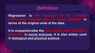
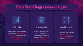
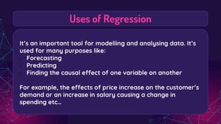
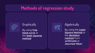
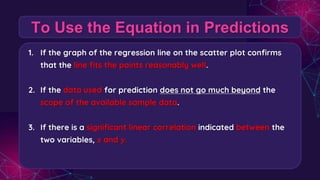
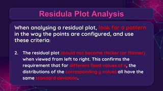
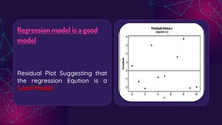
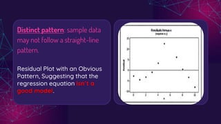
1. Analysis on
Simple Linear Regression
Presensted by:

2. TABLE OF CONTENTS
Key Concepts
Simple Linear
Regression
Example
01
02
03
04 Error - Residual

3. Key Concepts
01
Deffinition, prediction & benefits.

4. Definition
Regression is the measure of the average
relationship between two or more variables in
terms of the original units of the data.
It is unquestionable the most widely used statistical
technique in social sciences. It is also widely used
in biological and physical science.

5. Prediction using Regression analysis
Interpolation
If we give prediction within
the range of the given data
value
If we give prediction outside
the range of the given data
value
Extrapolation

6. Graphical difference

7. Relationship
Benefits of Regression analysis
Estimate
It provides estimate of
values of dependent
variables from values
of independent
variables
Extended
It can be extended
to 2 or more
variables, which is
known as multiple
regression
It shows the nature
of relationship
between two or
more variables

8. In the field of Business
The success of a
business depends on the
correctness of the
estimates in predicting
future production,
prices, profits, sales etc.

9. It’s an important tool for modelling and analysing data. It’s
used for many purposes like:
● Forecasting
● Predicting
● Finding the causal effect of one variable on another
For example, the effects of price increase on the customer’s
demand or an increase in salary causing a change in
spending etc…
Uses of Regression

10. Simple Linear
Regression
02
Requirements, Methods, Equation & Parameters.

11. Requirements
• The sample of paired data is a simple random
sample of quantitative data.
• The pairs of data 𝑥, 𝑦 have a bivariate normal
distribution, meaning the following:
- Visual examination of the scatter plot
confirms that the sample points follow an
approximately straight line.
- No Outliners.

12. Methods of regression study
Graphically
By using free
hand curve or
the least squares
method
Algebrically
By using the Least
Square Method or
the deviation
method from
arithmatic or
Assumed Mean

13. The Linear Equation
Y = a + bX
Where
Y = dependent variable
X = independent variable
a = constant (value of Y when X = 0)
b = the slope of the regression line

14. Least Square Method
∑𝒀 = 𝒏𝒂 + 𝒃∑𝑿
∑𝑿𝒀 = 𝒂∑𝑿 + 𝒃∑𝑿𝟐
The values of a and b are found with the
help of least of Squares-reference
method’s normal equations
Y=Dependent variable
X=Independent variable
Y = a + b X
01
02
03

15. Equation parameters
“a”
• a is the point at which the
slope line passes through the
Y axis.
• can be positive or negative
• may be referred to a as the
intercept.
“b”
• (the slope coefficient)
• can be positive or
negative.
• denotes a positive
or negative relationship.

16. Example 03
Solving equations to determine
parameters and using it in prediction

17. Preditction
Example
Using Variable x to
predict the response of
variable y
X 3 2 7 4 8
Y 6 1 8 5 9

18. Example
X Y XY 𝐗𝟐
3 6 18 9
2 1 2 4
7 8 56 49
4 5 20 16
8 9 72 64

19. Example
The Intercept
a = 0.66
The Slope
b = 1.07
By solving the equations

20. Regression
Equation and Graph
𝒀 = 𝟎. 𝟔𝟔 + 𝟏. 𝟎𝟕𝑿

21. To Use the Equation in Predictions
1. If the graph of the regression line on the scatter plot confirms
that the line fits the points reasonably well.
2. If the data used for prediction does not go much beyond the
scope of the available sample data.
3. If there is a significant linear correlation indicated between the
two variables, 𝑥 and 𝑦.

22. Residuals 04
Errors

23. Residual - Error
Residual – for a pair of sample 𝑥 and 𝑦 values, the difference
between the observed sample value of 𝑦 (a true value observed)
and the y-value that is predicted by using the regression equation 𝑦
is the residual
• 𝑅𝑒𝑠𝑖𝑑𝑢𝑎𝑙 = 𝑂𝑏𝑠𝑒𝑟𝑣𝑒𝑑 - 𝑃𝑟𝑒𝑑𝑖𝑐𝑡𝑒𝑑
= 𝒀𝑶𝒃𝒔𝒆𝒓𝒗𝒆𝒅 - 𝒀𝑷𝒓𝒆𝒅𝒊𝒄𝒕𝒆𝒅
• A residual represents a type of inherent prediction error
• The regression equation does not, typically, pass through all the
observed data values that we have

24. Residual - Error

25. Residual Plot
Residual Plot – a scatter plot of the 𝑥, 𝑦 values after each
of the y-values has been replaced by the residual
value, “𝒀𝑶𝒃𝒔𝒆𝒓𝒗𝒆𝒅 - 𝒀𝑷𝒓𝒆𝒅𝒊𝒄𝒕𝒆𝒅”
• That is, a residual plot is a graph of the points
𝑥, ( 𝒀𝑶𝒃𝒔𝒆𝒓𝒗𝒆𝒅 - 𝒀𝑷𝒓𝒆𝒅𝒊𝒄𝒕𝒆𝒅 )

26. Residula Plot Analysis
When analysing a residual plot, look for a pattern
in the way the points are configured, and use
these criteria:
1. The residual plot should not have any obvious patterns
(not even a straight line pattern). This confirms that the
scatterplot of the sample data is a straight-line pattern.

27. Residula Plot Analysis
When analysing a residual plot, look for a pattern
in the way the points are configured, and use
these criteria:
2. The residual plot should not become thicker (or thinner)
when viewed from left to right. This confirms the
requirement that for different fixed values of x, the
distributions of the corresponding y values all have the
same standard deviation.

28. Let’s observe what is good or bad
about the individual regression
models.

29. Regression model is a good
model
Residual Plot Suggesting that
the regression Eqution is a
Good Model

30. Distinct pattern: sample data
may not follow a straight-line
pattern.
Residual Plot with an Obvious
Pattern, Suggesting that the
regression equation Isn’t a
good model.

31. Residual plot becoming
thicker: equal standard
deviations violated
Residual Plot that becomes
thicker. Suggesting that the
regression equation Isn’t a
good model

32. CREDITS: This presentation template was
created by Slidesgo, including icons by
Flaticon, and infographics & images by
Freepik
Many
Thanks!
Presented by: