signal and system

SIGNALS & SYSTEMS (2141005) EXPERIMENT- 1
ELECTRICALDEPARTMENT
BITS EDU CAMPUS Page 1
Babaria Institute of Technology
Electrical Engineering Department
Semester :4 Branch:EE
Subject: Signals & Systems (2141005) Experiment No. 1
Aim: To familiarize with MATLAB software, general functions and signal processing
toolbox functions.
The name MATLAB stands for MATrix LABoratory produced by Mathworks Inc., USA. It is a
matrix-based powerful software package for scientific and engineering computation and
visualization. Complex numerical problems can be solved in a fraction of the time that
required with other high level languages. It provides an interactive environment with
hundreds of built -in –functions for technical computation, graphics and animation. In
addition to built-in-functions, user can create his own functions.
MATLAB offers several optional toolboxes, such as signal processing, control systems, neural
networks etc. It is command driven software and has online help facility.
MATLAB has three basic windows normally; command window, graphics window and edit
window.
Command window is characterized by the prompt ‘>>’.
All commands and the ready to run program filename can be typed here. Graphic window
gives the display of the figures as the result of the program. Edit window is to create
program files with an extension .m.
Some important commands in MATLAB
Help : List topics on which help is available
Help command name: Provides help on the topic selected
Demo : Runs the demo program
Who : Lists variables currently in the workspace
Whos : Lists variables currently in the workspace with their size
Clear : Clears the workspace, all the variables are removed
Clear x,y,z : Clears only variables x,y,z
Quit: Quits MATLAB

Some of the frequently used built-in-functions in Signal Processing Toolbox
filter(b.a.x): Syntax of this function is Y = filter(b.a.x)
It filters the data in vector x with the filter described by vectors
a and b to create the filtered data y.
fft (x): It is the DFT of vector x
ifft (x) : It is the DFT of vector x
conv (a,b) : Syntax of this function is C = conv (a,b)
It convolves vectors a and b. The resulting vector is ofLength,
Length (a) + Length (b)-1
deconv(b,a): Syntax of this function is [q,r] = deconv(b,a)
It deconvolves vector q and the remainder in vector r such that
b = conv(a,q)+r
butter(N,Wn): Designs an Nth order lowpass digital Butterworth filter and
returns the filter coefficients in length N+1 vectors B
(numerator) and A (denominator). The coefficients are listed in
descending powers of z. The cutoff frequency Wn must be 0.0
< Wn < 1.0, with 1.0 corresponding tohalf the sample rate.
buttord(Wp, Ws, Rp, Rs): Returns the order N of the lowest order digital Butterworth
filter that loses no more than Rp dB in the passband and has at
least Rs dB of attenuation in the stopband. Wp and Ws are the
passband and stopband edge frequencies, Normalized from 0
to 1 ,(where 1 corresponds to pi rad/sec)
Cheby1(N,R,Wn) : Designs an Nth order lowpass digital Chebyshev filter with R
decibels of peak-to-peak ripple in the passband. CHEBY1
returns the filter coefficients in length N+1 vectors B
(numerator) and A (denominator). The cutoff frequency Wn
must be 0.0 < Wn < 1.0, with 1.0 corresponding to half the
sample rate.
Cheby1(N,R,Wn,'high'): Designs a highpass filter.

Cheb1ord(Wp, Ws, Rp, Rs): Returns the order N of the lowest order digital Chebyshev
Type I filter that loses no more than Rp dBin the passband and
has at least Rs dB of attenuation in the stopband. Wp and Ws
are the passband and stopband edge frequencies, normalized
from 0 to 1 (where 1 corresponds to pi radians/sample)
cheby2(N,R,Wn) : Designs an Nth order lowpass digital Chebyshev filter with the
stopband ripple R decibels down and stopband edge
frequency Wn. CHEBY2 returns the filter coefficients in length
N+1 vectors B (numerator) and A. The cutoff frequency Wn
must be 0.0 < Wn < 1.0, with 1.0 corresponding to half the
sample rate.
cheb2ord(Wp, Ws, Rp, Rs): Returns the order N of the lowest order digital Chebyshev
Type II filter that loses no more than Rp dB in the passband
and has at least Rs dB of attenuation in the stopband. Wp and
Ws are the passband and stopband edge frequencies.
abs(x): It gives the absolute value of the elements of x. When x is
complex, abs(x) is the complex modulus (magnitude) of the
elements of x.
angle(H): It returns the phase angles of a matrix with complex elements
in
radians.
freqz(b,a,N) : Syntax of this function is [h,w] = freqz(b,a,N) returns the
Npoint
frequency vector w in radians and the N-point complex
frequency response vector h of the filter b/a.
stem(y) : It plots the data sequence y aa stems from the x axis
terminated
with circles for the data value.
stem(x,y): It plots the data sequence y at the values specified in x.
ploy(x,y) : It plots vector y versus vector x. If x or y is a matrix, then the
vector is plotted versus the rows or columns of the
matrix,cwhichever line up.
title(‘text’): It adds text at the top of the current axis.
xlabel(‘text’): It adds text beside the x-axis on the current axis.
ylabel(‘text’): It adds text beside the y-axis on the current axis.

Experiment :2
To plot graph of Continuous Time Signals

Unit step function
Program :
T=30;
x=ones(1,T);
t=0:1:T-1
plot(t,x);
grid on;
xlabel('time(sec)')
ylabel('x(t)')
Output :
0 5 10 15 20 25 30
0
0.5
1
1.5
2
time(sec)
x(t)

Unit ramp function
Program :
t=0:0.03:4;
x=t;
plot(t,x)
grid on;
xlabel('Time(sec)')
ylabel('x(t)')
Output :
0 1 2 3 4
0
1
2
3
4
Time(sec)
x(t)

Unit parabolic function
Program :
t=0:0.01:2;
x=t.^2/2;
plot(t,x);
grid on;
xlabel('Time(sec)')
ylabel('x(t)')
Output :
0 0.5 1 1.5 2
0
0.5
1
1.5
2
Time(sec)
x(t)

Impulse function
Program :
for t = 0;
x = 1;
end;
plot(t,x);
stem(t,x)
grid on;
xlabel('Time(sec)')
ylabel('x(t)')
Output :
-1 -0.5 0 0.5 1
0
0.2
0.4
0.6
0.8
1
Time(sec)
x(t)

Rectangular pulse function
Program :
t=-1:0.001:1;
x=rectpuls(t);
plot(t,x);
grid on;
xlabel('Time(sec)')
ylabel('x(t)')
Output :
-1 -0.5 0 0.5 1
0
0.2
0.4
0.6
0.8
1
Time(sec)
x(t)

Triangular pulse function
Program :
t=-1:0.002:1;
x=tripuls(t);
plot(t,x);
grid on;
xlabel('Time(sec)')
ylabel('x(t)')
Output:
Signum function
-1 -0.5 0 0.5 1
0
0.2
0.4
0.6
0.8
1
Time(sec)
x(t)

Program :
t=-10:0.001:10;
x=sign(t);
plot(t,x);
grid on;
xlabel('Time(sec)')
ylabel('x(t)')
Output:
-10 -5 0 5 10
-1
-0.5
0
0.5
1
Time(sec)
x(t)

Sinc function
Program :
t =-4:0.05:4;
x=sinc(t);
plot(t,x);
grid on;
xlabel('Time(sec)')
ylabel('x(t)')
Output:
-4 -2 0 2 4
-0.4
-0.2
0
0.2
0.4
0.6
0.8
1
Time(sec)
x(t)

Gaussian function
Program :
t=-5:0.03:5;
a=1;
x=exp(-a*t.^2);
plot(t,x)
grid on;
xlabel('Time(sec)')
ylabel('x(t)')
Output :
-5 0 5
0
0.2
0.4
0.6
0.8
1
Time(sec)
x(t)

Sinusoidal signal
Program :
t=0:0.01:2;
x=2*sin(pi*t);
plot(t,x);
grid on;
xlabel('Time(sec)')
ylabel('x(t)')
Output :
0 0.5 1 1.5 2
-2
-1
0
1
2
Time(sec)
x(t)

Real exponential signals
Program :
t=0:0.04:4;
x=2*exp(1*t);
plot(t,x);
grid on;
xlabel('Time(sec)')
ylabel('x(t)')
Output : 1. a>0
0 1 2 3 4
0
10
20
30
40
50
60
Time(sec)
x(t)

Program :
t=0:0.04:4;
x=2*exp(-1*t);
plot(t,x);
grid on;
xlabel('Time(sec)')
ylabel('x(t)')
Output : 2. a<0
Program :
0 1 2 3 4
0
0.2
0.4
0.6
0.8
1
Time(sec)
x(t)

t=0:0.04:4;
x=2*exp(0*t);
plot(t,x);
grid on;
xlabel('Time(sec)')
ylabel('x(t)')
Output : 3. a=0
0 1 2 3 4
-1
-0.5
0
0.5
1
Time(sec)
x(t)

Complex exponential function
Program :
t=-10:0.001:10;
c=complex(0,1);
x=exp(c*t);
plot(t,x);
grid on;
xlabel('Time(sec)')
ylabel('x(t)')
Output :
-10 -5 0 5 10
-1
-0.5
0
0.5
1
Time(sec)
x(t)

Program :
t=-10:0.001:10;
c=complex(-1,12);
x=exp(c*t);
plot(t,x);
grid on;
xlabel('Time(sec)')
ylabel('x(t)')
Output :
-10 -5 0 5 10
-2
-1
0
1
2
3
x 10
4
Time(sec)
x(t)

Program :
t=-10:0.001:10;
c=complex(1,12);
x=exp(c*t);
plot(t,x);
grid on;
xlabel('Time(sec)')
ylabel('x(t)')
Output :
-10 -5 0 5 10
-2
-1
0
1
2
3
x 10
4
Time(sec)
x(t)

Experiment :3
To plot graph of Discrete Time Signals

Unit step sequence
Program :
T=30;
x=ones(1,T);
t=0:1:T-1
stem(t,x);
grid on;
xlabel('time(sec)')
ylabel('x(t)')
Output :
0 5 10 15 20 25 30
0
0.2
0.4
0.6
0.8
1
time(sec)
x(t)

Unit ramp sequence
Program :
t=0:0.5:4;
x=t;
stem(t,x);
grid on;
xlabel('Time(sec)')
ylabel('x(t)')
Output :
0 1 2 3 4
0
1
2
3
4
Time(sec)
x(t)

Unit impulse sequence
Program :
for t = 0;
x = 1;
end;
plot(t,x);
stem(t,x)
grid on;
xlabel('Time(sec)')
ylabel('x(t)')
Output :
-1 -0.5 0 0.5 1
0
0.2
0.4
0.6
0.8
1
Time(sec)
x(t)

Exponential sequence
Program :
t=0:0.35:4;
x=2.^t;
stem(t,x);
grid on;
xlabel('Time(sec)')
ylabel('x(t)')
Output :
0 1 2 3 4
0
10
20
30
40
50
Time(sec)
x(t)

Program :
t=0:0.35:4;
x=0.2.^t;
stem(t,x);
grid on;
xlabel('Time(sec)')
ylabel('x(t)')
Output :
0 1 2 3 4
0
0.2
0.4
0.6
0.8
1
Time(sec)
x(t)

Program :
t=0:0.35:4;
x=-0.2.^t;
stem(t,x);
grid on;
xlabel('Time(sec)')
ylabel('x(t)')
Output :
0 1 2 3 4
-1
-0.8
-0.6
-0.4
-0.2
0
Time(sec)
x(t)

Program :
t=0:0.35:4;
x=-2.^t;
stem(t,x);
grid on;
xlabel('Time(sec)')
ylabel('x(t)')
Output :
0 1 2 3 4
-15
-10
-5
0
Time(sec)
x(t)

Sinusoidal sequence
Program :
t=0:0.1:2;
x=2*sin(pi*t);
stem(t,x);
grid on;
xlabel('Time(sec)')
ylabel('x(t)')
Output :
0 0.5 1 1.5 2
-2
-1
0
1
2
Time(sec)
x(t)

Complex exponential sequence
Program :
t=-10:0.3:10;
c=complex(0.3,4);
x=exp(c*t);
stem(t,x);
grid on;
xlabel('Time(sec)')
ylabel('x(t)')
Output :
-10 -5 0 5 10
-15
-10
-5
0
5
10
15
20
Time(sec)
x(t)

Program :
t=-10:0.3:10;
c=complex(0.3,4);
x=exp(c*t);
stem(t,x);
grid on;
xlabel('Time(sec)')
ylabel('x(t)')
Output :
-10 -5 0 5 10
-15
-10
-5
0
5
10
15
20
Time(sec)
x(t)

Experiment :04
To perform signal operation using
stimulink

Program : u(t)-u(t-1)
Output :

Program : r(t)-2r(t-1)+r(t-2)
Output :

Program : r(t)-2u(t-1)-r(t-2)
Output :

Program : r(t)-r(t-1)-u(t-1)
Output :

Experiment :05
To perform the convolution sum
of discrete time signal.

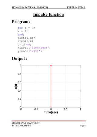
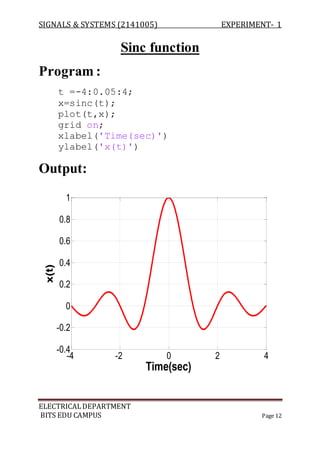
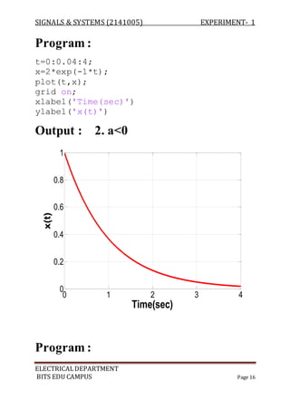
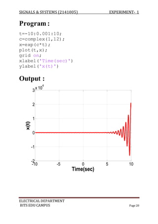
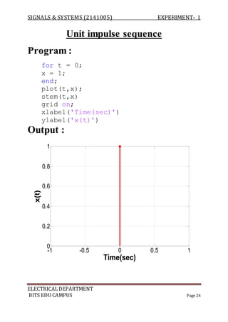
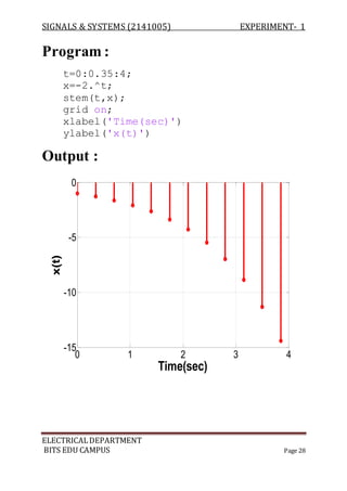
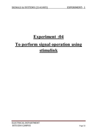
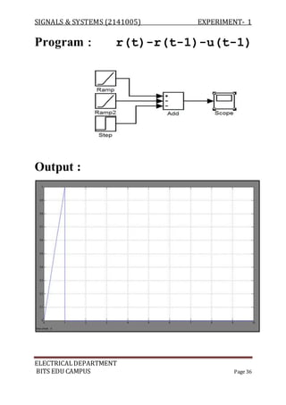
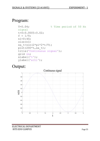
Program :
a=[ 1 -1 2 3];
b=[ 1 -2 3 -1];
z=conv(a,b);
m=length(z);
y=0:m-1;
stem(y,z);
Output :
0 1 2 3 4 5 6
-5
0
5
10
a
b

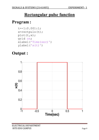
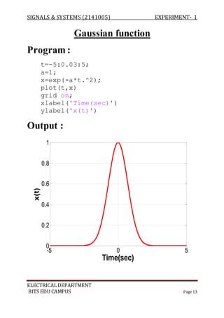
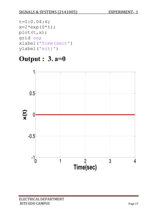
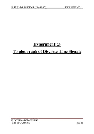
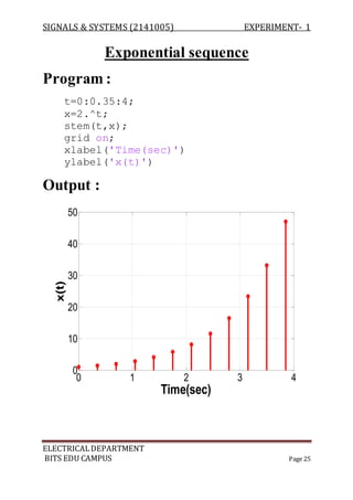
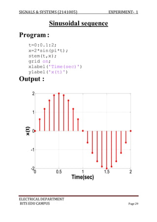
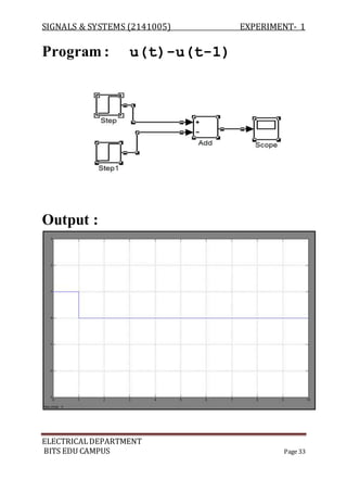
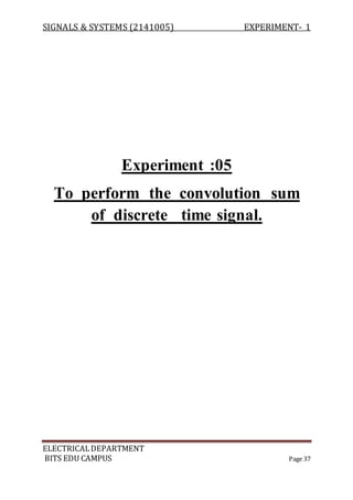
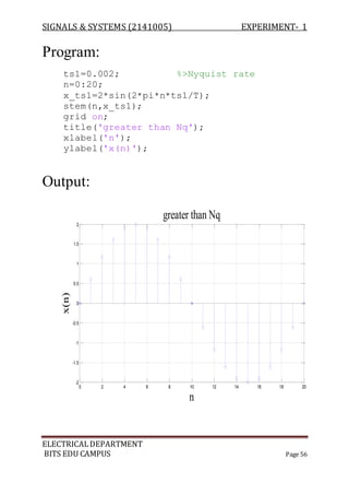
Program :
a=[ 1 2 3 2];
b=[ 1 2 2];
z=conv(a,b);
m=length(z);
y=0:m-1;
stem(y,z);
Output :
0 0.5 1 1.5 2 2.5 3 3.5 4 4.5 5
0
5
10
15
a
b

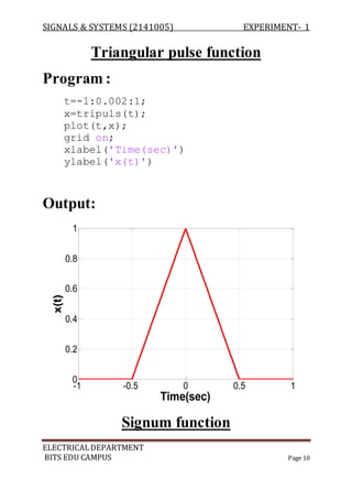
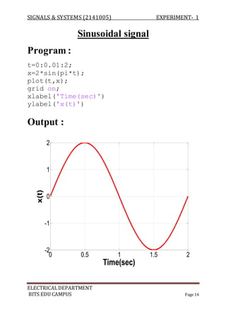
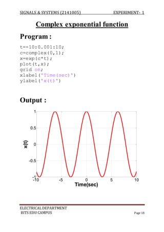
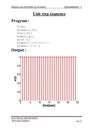
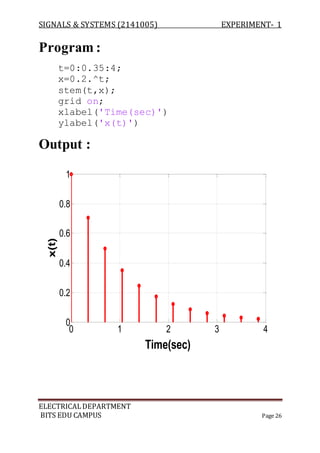
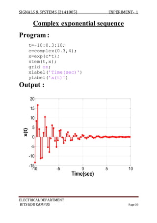
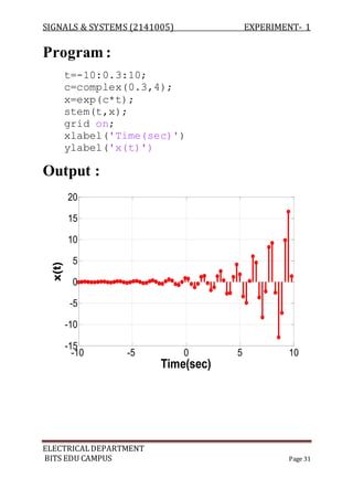
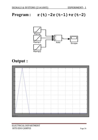
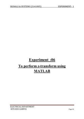
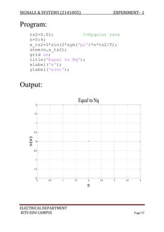
Program :
a=[ 1 4 3 2];
b=[ 1 3 2 1];
z=conv(a,b);
m=length(z);
y=0:m-1;
stem(y,z);
Output :
0 1 2 3 4 5 6
0
5
10
15
20
a
b

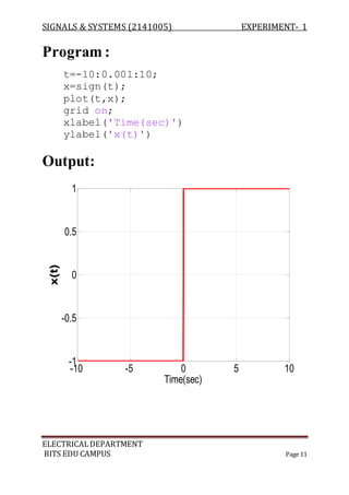
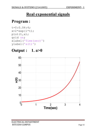
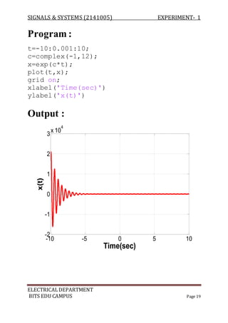
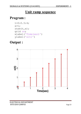
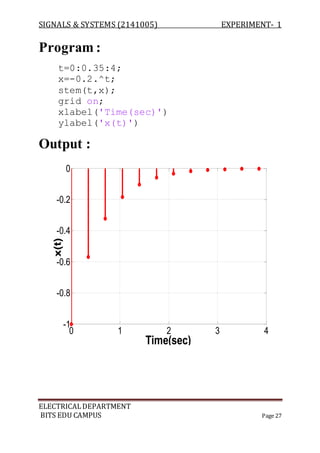
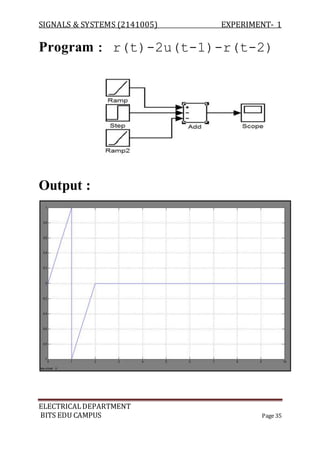
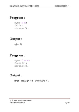
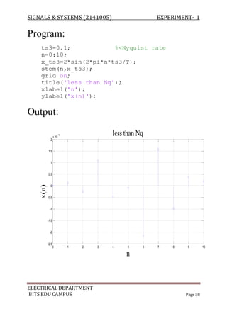
Program:
a=[ 1 -2 3 1];
b=[ 2 -3 -2];
z=conv(a,b);
m=length(z);
y=0:m-1;
stem(y,z);
Output:
0 0.5 1 1.5 2 2.5 3 3.5 4 4.5 5
-10
-5
0
5
10
a
b

Experiment :06
To perform z-transform using
MATLAB

Program :
syms f n;
f=2^n;
ztrans(f);
Output :
z/(z - 2)
Program :
syms f n w;
f=cos(n);
ztrans(f);
Output :
(z*(z - cos(1)))/(z^2 - 2*cos(1)*z + 1)

Program :
syms f n w;
f=2^n+3^n;
ztrans(f);
Output :
z/(z - 2) + z/(z - 3)
Program :
syms f n w;
f=(n^2)*(2^n);
ztrans(f);
Output :
(z^2/4 + z/2)/(z/2 - 1)^3

Experiment :07
To plot zeros and poles in the z-plane
using MATLAB.

Program :
syms n d z
n=[1 1];
d=[1 2 3 4];
sys=tf(n,d),disp(z);
zplane(n,d);
Output :
s + 1
s^3 + 2 s^2 + 3 s + 4
-2 -1.5 -1 -0.5 0 0.5 1 1.5
-1.5
-1
-0.5
0
0.5
1
1.5
2
Real Part
ImaginaryPart

Program :
syms n d z
n=[1 0.5];
d=[1 1 1];
zplane(n,d);
Output :
s + 0.5
s^2 + s + 1
-1.5 -1 -0.5 0 0.5 1 1.5
-1
-0.5
0
0.5
1
Real Part
ImaginaryPart

Program :
syms n d z
n=[3 0];
d=[1 6 9];
zplane(n,d);
Output :
3 s
s^2 + 6 s + 9
-3 -2 -1 0 1
-1
-0.5
0
0.5
1
22
Real Part
ImaginaryPart

Program :
syms n d z
n=[1 1 0];
d=[1 3 1 1];
zplane(n,d);
Output :
s^2 + s
s^3 + 3 s^2 + s + 1
-2.5 -2 -1.5 -1 -0.5 0 0.5 1
-1
-0.5
0
0.5
1
2
Real Part
ImaginaryPart

Experiment -08
To perform FFT using MATLAB.

1. Program:
a = input('enter sequence');
b = length(a);
x = fft(a,b)
Output:
Enter sequence[1 2 3 4]
x =
10.0000 -2.0000 + 2.0000i -2.0000 -2.0000 - 2.0000i
2. Program :
a = input('enter sequence');
b = length(a);
x = fft(a,b)
Output :
enter sequence[5 7 9 5]
x =
26.0000 -4.0000 - 2.0000i 2.0000
-4.0000 + 2.0000i

Experiment -09
To perform IFFT using MATLAB.

1. Program:
a = input('Enter sequence');
b = length(a);
x = ifft(a,b)
Output:
x =
2.5000 -0.5000 - 0.5000i -0.5000
-0.5000 + 0.5000i
2. Program :
a = input('Enter sequence');
b = length(a);
x = ifft(a,b)
Output:
x =
5.2500 -1.5000 - 0.2500i -0.2500
-1.5000 + 0.2500i

Experiment - 10
To verify sampling theorem using
MATLAB.

Program:
T=0.04; % Time period of 50 Hz
signal
t=0:0.0005:0.02;
f = 1/T;
n1=0:40;
size(n1)
xa_t=sin(2*pi*2*t/T);
plot(200*t,xa_t);
title('Continuous signal');
grid on;
xlabel('t');
ylabel('x(t)');
Output:
0 0.5 1 1.5 2 2.5 3 3.5 4
-1
-0.8
-0.6
-0.4
-0.2
0
0.2
0.4
0.6
0.8
1
Continuous signal
t
x(t)

Program:
ts1=0.002; %>Nyquist rate
n=0:20;
x_ts1=2*sin(2*pi*n*ts1/T);
stem(n,x_ts1);
grid on;
title('greater than Nq');
xlabel('n');
ylabel('x(n)');
Output:
0 2 4 6 8 10 12 14 16 18 20
-2
-1.5
-1
-0.5
0
0.5
1
1.5
2
greater than Nq
n
x(n)

Program:
ts2=0.01; %=Nyquist rate
n=0:4;
x_ts2=2*sin(2*sym('pi')*n*ts2/T);
stem(n,x_ts2);
grid on;
title('Equal to Nq');
xlabel('n');
ylabel('x(n)');
Output:
0 0.5 1 1.5 2 2.5 3 3.5 4
-2
-1.5
-1
-0.5
0
0.5
1
1.5
2
Equal to Nq
n
x(n)

Program:
ts3=0.1; %<Nyquist rate
n=0:10;
x_ts3=2*sin(2*pi*n*ts3/T);
stem(n,x_ts3);
grid on;
title('less than Nq');
xlabel('n');
ylabel('x(n)');
Output:
0 1 2 3 4 5 6 7 8 9 10
-2.5
-2
-1.5
-1
-0.5
0
0.5
1
1.5
2
x 10
-14 less than Nq
n
x(n)

signal and system

Recommended

Recommended

More Related Content

What's hot

What's hot (20)

Similar to signal and system

Similar to signal and system (20)

More from SAURAV DAYAL SING

More from SAURAV DAYAL SING (7)

Recently uploaded

Recently uploaded (20)

signal and system