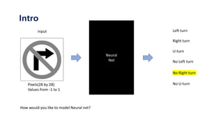
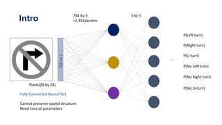
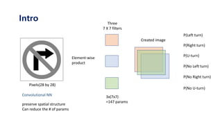
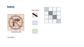
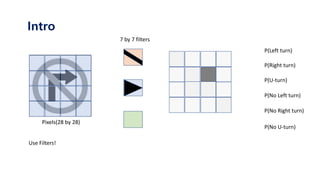
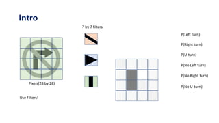
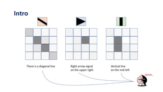
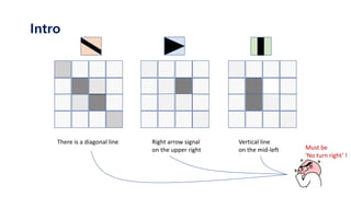
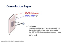
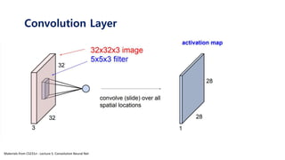
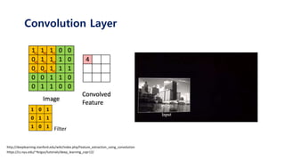
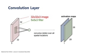
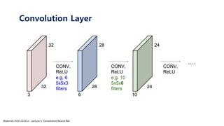
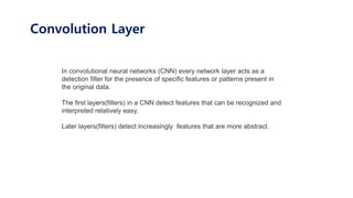
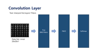
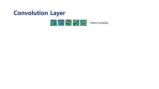
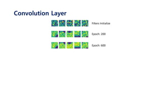
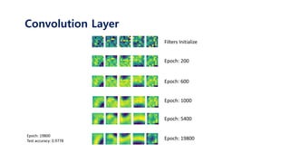
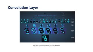
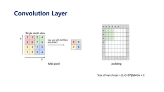
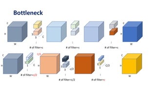
The document serves as a tutorial on convolutional neural networks (CNNs), covering their architecture, implementation, and functionality. It discusses key concepts such as convolution layers, backpropagation, and the role of filters in detecting features at various abstraction levels. Various examples and code snippets are provided to illustrate the practical aspects of CNNs, emphasizing the importance of efficient parameter usage and feature extraction.
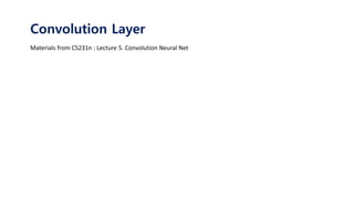

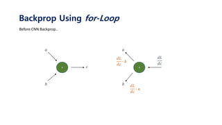
![conv
𝑥 1
𝑊 1
𝑎 1
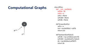
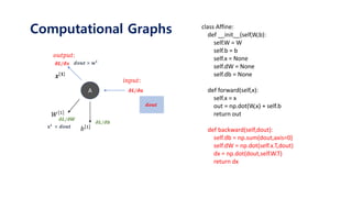
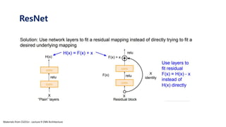
def forward(self,x):
self.x = x
#input과 filter의 column(=row) 크기 계산
size_x = self.x.shape[0]
size_W = self.W.shape[0]
#convolution 크기 계산후 생성 (x-w)/stride + 1
size_c = size_x - size_W + 1
conv_result = np.zeros(shape=(size_c,size_c))
#합성곱 연산
for i in range(size_c) :
for j in range(size_c):
partial = x[i:i+size_W , j:j+size_W]
conv_result[i][j] = partial * size_W
return conv_result
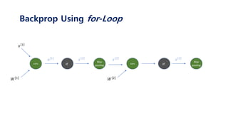
Backprop Using for-Loop](https://image.slidesharecdn.com/tutorialonconvolutionalneuralnetworks-180202150458/85/Tutorial-on-convolutional-neural-networks-39-320.jpg)
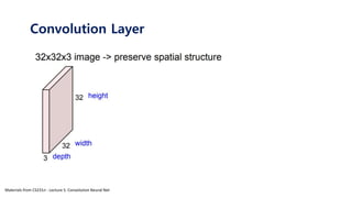
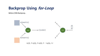
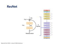
![conv
𝑥 1
𝑊 1
𝑎 1
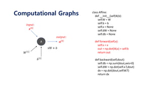
def forward(self,x):
self.x = x
#input과 filter의 column(=row) 크기 계산
size_x = self.x.shape[0]
size_W = self.W.shape[0]
#convolution 크기 계산후 생성 (x-w)/stride + 1
size_c = size_x - size_W + 1
conv_result = np.zeros(shape=(size_c,size_c))
#합성곱 연산
for i in range(size_c) :
for j in range(size_c):
partial = x[i:i+size_W , j:j+size_W]
conv_result[i][j] = partial * size_W
return conv_result
Backprop Using for-Loop](https://image.slidesharecdn.com/tutorialonconvolutionalneuralnetworks-180202150458/85/Tutorial-on-convolutional-neural-networks-40-320.jpg)
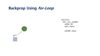
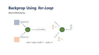
![conv
𝑥 1
𝑊 1
𝑎 1
def forward(self,x):
self.x = x
#input과 filter의 column(=row) 크기 계산
size_x = self.x.shape[0]
size_W = self.W.shape[0]
#convolution 크기 계산후 생성 (x-w)/stride + 1
size_c = size_x - size_W + 1
conv_result = np.zeros(shape=(size_c,size_c))
#합성곱 연산
for i in range(size_c) :
for j in range(size_c):
partial = x[i:i+size_W , j:j+size_W]
conv_result[i][j] = partial * size_W
return conv_result
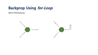
Backprop Using for-Loop](https://image.slidesharecdn.com/tutorialonconvolutionalneuralnetworks-180202150458/85/Tutorial-on-convolutional-neural-networks-41-320.jpg)
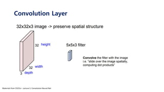
![conv
𝑥 1
𝑊 1
𝑎 1
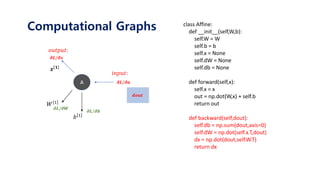
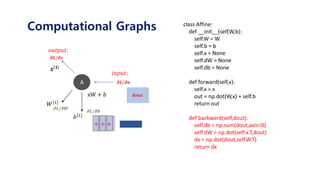
def backward(self, dout):
#input과 filter,x의 column(=row) 크기 계산
size_x = self.x.shape[0] #column(=row) 크기
size_W = self.W.shape[0]
size_dout = dout.shape[0]
#filter의 미분 결과 matrix
self.dW = np.zeros(shape=(size_W,size_W))
#x의 미분 결과 matrix
dx = np.zeros(shape=(size_x,size_x))
for i in range(size_dout) :
for j in range(size_dout) :
partial = self.x[i:i+size_W, j:j+size_W]
self.dW += dout[i][j] * partial
dx[i:i+size_W,j:j+size+W] += dout[i][j] * self.W
return dx
Backprop Using for-Loop](https://image.slidesharecdn.com/tutorialonconvolutionalneuralnetworks-180202150458/85/Tutorial-on-convolutional-neural-networks-46-320.jpg)
![conv
𝑥 1
𝑊 1
𝑎 1
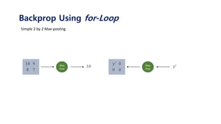
Backprop Using for-Loop
def backward(self, dout):
#input과 filter,x의 column(=row) 크기 계산
size_x = self.x.shape[0] #column(=row) 크기
size_W = self.W.shape[0]
size_dout = dout.shape[0]
#filter의 미분 결과 matrix
self.dW = np.zeros(shape=(size_W,size_W))
#x의 미분 결과 matrix
dx = np.zeros(shape=(size_x,size_x))
for i in range(size_dout) :
for j in range(size_dout) :
partial = self.x[i:i+size_W, j:j+size_W]
self.dW += dout[i][j] * partial
dx[i:i+size_W,j:j+size+W] += dout[i][j] * self.W
return dx](https://image.slidesharecdn.com/tutorialonconvolutionalneuralnetworks-180202150458/85/Tutorial-on-convolutional-neural-networks-47-320.jpg)
![conv
𝑥 1
𝑊 1
𝑎 1
Backprop Using for-Loop
def backward(self, dout):
#input과 filter,x의 column(=row) 크기 계산
size_x = self.x.shape[0] #column(=row) 크기
size_W = self.W.shape[0]
size_dout = dout.shape[0]
#filter의 미분 결과 matrix
self.dW = np.zeros(shape=(size_W,size_W))
#x의 미분 결과 matrix
dx = np.zeros(shape=(size_x,size_x))
for i in range(size_dout) :
for j in range(size_dout) :
partial = self.x[i:i+size_W, j:j+size_W]
self.dW += dout[i][j] * partial
dx[i:i+size_W,j:j+size+W] += dout[i][j] * self.W
return dx](https://image.slidesharecdn.com/tutorialonconvolutionalneuralnetworks-180202150458/85/Tutorial-on-convolutional-neural-networks-48-320.jpg)
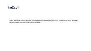
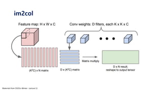
![im2col def im2col(input_data, filter_h, filter_w, stride=1, pad=0):
"""다수의 이미지를 입력받아 2차원 배열로 변환한다(평탄화).
Parameters
----------
input_data : 4차원 배열 형태의 입력 데이터(이미지 수, 채널 수, 높이, 너비)
filter_h : 필터의 높이
filter_w : 필터의 너비
stride : 스트라이드
pad : 패딩
Returns
-------
col : 2차원 배열
"""
N, C, H, W = input_data.shape
out_h = (H + 2*pad - filter_h)//stride + 1
out_w = (W + 2*pad - filter_w)//stride + 1
img = np.pad(input_data, [(0,0), (0,0), (pad, pad), (pad, pad)], 'constant')
col = np.zeros((N, C, filter_h, filter_w, out_h, out_w))
for y in range(filter_h):
y_max = y + stride*out_h
for x in range(filter_w):
x_max = x + stride*out_w
col[:, :, y, x, :, :] = img[:, :, y:y_max:stride, x:x_max:stride]
col = col.transpose(0, 4, 5, 1, 2, 3).reshape(N*out_h*out_w, -1)
return col
https://github.com/WegraLee/deep-learning-from-scratch/blob/master/common/util.py](https://image.slidesharecdn.com/tutorialonconvolutionalneuralnetworks-180202150458/85/Tutorial-on-convolutional-neural-networks-51-320.jpg)


![[PR12] Inception and Xception - Jaejun Yoo](https://cdn.slidesharecdn.com/ss_thumbnails/pr12inceptionandxception-jaejunyoo-170910140157-thumbnail.jpg?width=640&height=640&fit=bounds)