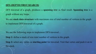
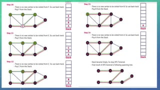
This document discusses graph traversal techniques for searching graphs. It describes two common techniques: breadth-first search (BFS) and depth-first search (DFS). BFS uses a queue data structure to visit all adjacent vertices of the starting vertex before moving to the next level, producing a spanning tree. DFS uses a stack, visiting all vertices reachable from the starting point before backtracking, also producing a spanning tree. The document outlines the step-by-step process for implementing BFS and DFS on a graph.

1. GRAPH TRAVERSALS IN DATA STRUCTURE
BY
D.SEETHALAKSHMI
ASSISTANT PROFESSOR
BON SECOURS COLLEGE FOR WOM EN

2. GRAPH TRAVERSALS
Graph traversal is technique used for searching a vertex in a graph. The graph traversal
is also used to decide the order of vertices to be visit in the search process.
A graph traversal finds the edges to be used in the search process without creating
loops that means using graph traversal we visit all vertices of graph without getting
into looping path.
There are two graph traversal techniques and they are as follows...
 BFS (breadth first search)
 DFS (depth first search)

3. BFS (Breadth First Search)
 BFS traversal of a graph, produces a spanning tree as final result.
 Spanning tree is a graph without any loops.
 We use queue data structure with maximum size of total number of vertices in the
graph to implement BFS traversal of a graph.
We use the following steps to implement BFS traversal.
Step 1: Define a queue of size total number of vertices in the graph.
Step 2: Select any vertex as starting point for traversal. Visit that vertex and insert it
into the queue.

4. Step 3: Visit all the adjacent vertices of the vertex which is at front of the queue which is
not visited and insert them into the queue.
Step 4: When there is no new vertex to be visit from the vertex at front of the queue then
delete that vertex from the queue.
Step 5: Repeat step 3 and 4 until queue becomes empty.
Step 6: When queue becomes empty, then produce final spanning tree by removing
unused edges from the graph.

7. DFS (DEPTH FIRST SEARCH)
DFS traversal of a graph, produces a spanning tree as final result. Spanning tree is a
graph without any loops.
We use stack data structure with maximum size of total number of vertices in the graph
to implement DFS traversal of a graph.
We use the following steps to implement DFS traversal...
Step 1: define a stack of size total number of vertices in the graph.
Step 2: select any vertex as starting point for traversal. Visit that vertex and push it on to
the stack.

8. Step 3: visit any one of the adjacent vertex of the vertex which is at top of the stack
which is not visited and push it on to the stack.
Step 4: repeat step 3 until there are no new vertex to be visit from the vertex on top of the
stack.
Step 5: when there is no new vertex to be visit then use back tracking and pop one
vertex from the stack.
Step 6: repeat steps 3, 4 and 5 until stack becomes empty.
Step 7: when stack becomes empty, then produce final spanning tree by removing unused
edges from the graph.
Back tracking is coming back to the vertex from which we came to current vertex.