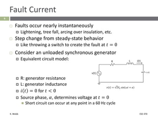
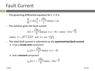
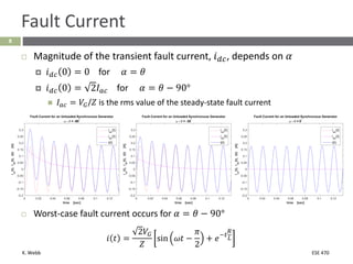
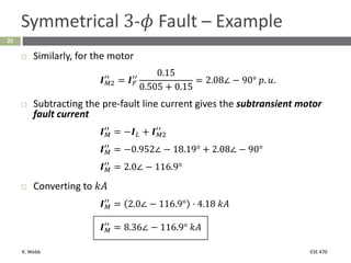
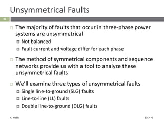
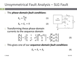
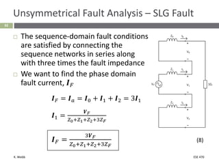
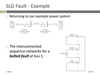
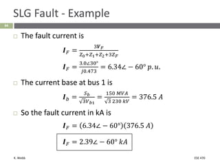
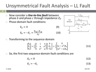
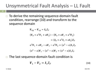
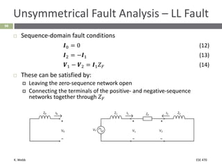
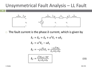
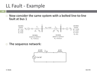
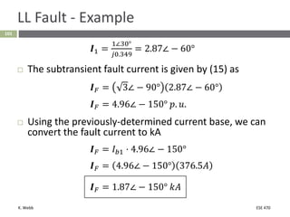
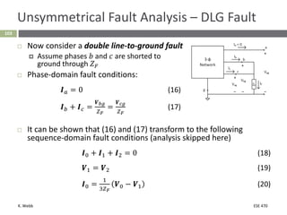
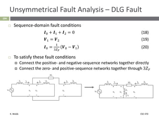
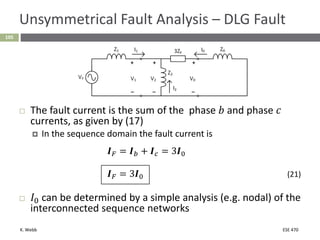
This document section discusses fault analysis in power systems. It begins by defining different types of faults like line-to-ground and line-to-line faults that can result in excessive current. It then discusses fault current calculations for a symmetrical three-phase fault on a simple system using superposition and per-unit calculations. As an example, it calculates the subtransient fault current, generator current, and motor current for a bolted three-phase fault at a bus.
3. K. Webb ESE 470
3
Power System Faults
Faults in three-phase power systems are short circuits
Line-to-ground
Line-to-line
Result in the flow of excessive current
Damage to equipment
Heat – burning/melting
Structural damage due to large magnetic forces
Bolted short circuits
True short circuits – i.e., zero impedance
In general, fault impedance may be non-zero
Faults may be opens as well
We’ll focus on short circuits
4. K. Webb ESE 470
4
Types of Faults
Type of faults from most to least common:
Single line-to-ground faults
Line-to-line faults
Double line-to-ground faults
Balanced three-phase (symmetrical) faults
We’ll look first at the least common type of fault –
the symmetrical fault – due to its simplicity
6. K. Webb ESE 470
6
Fault Current
R: generator resistance
L: generator inductance
𝑖 𝑡 = 0 for 𝑡 < 0
Source phase, 𝛼, determines voltage at 𝑡 = 0
Short circuit can occur at any point in a 60 Hz cycle
Faults occur nearly instantaneously
Lightening, tree fall, arcing over insulation, etc.
Step change from steady-state behavior
Like throwing a switch to create the fault at 𝑡 = 0
Consider an unloaded synchronous generator
Equivalent circuit model:
𝑣 𝑡 = 2𝑉𝐺 sin 𝜔𝑡 + 𝛼
7. K. Webb ESE 470
7
Fault Current
The governing differential equation for 𝑡 > 0 is
𝑑𝑖
𝑑𝑡
+ 𝑖 𝑡
𝑅
𝐿
=
2𝑉𝐺
𝐿
sin 𝜔𝑡 + 𝛼
The solution gives the fault current
𝑖 𝑡 =
2𝑉𝐺
𝑍
sin 𝜔𝑡 + 𝛼 − 𝜃 − sin 𝛼 − 𝜃 𝑒−𝑡
𝑅
𝐿
where 𝑍 = 𝑅2 + 𝜔𝐿 2 and 𝜃 = tan−1 𝜔𝐿
𝑅
This total fault current is referred to as the asymmetrical fault current
It has a steady-state component
𝑖𝑎𝑐 𝑡 =
2𝑉𝐺
𝑍
sin 𝜔𝑡 + 𝛼 − 𝜃
And a transient component
𝑖𝑑𝑐 𝑡 = −
2𝑉𝐺
𝑍
sin 𝛼 − 𝜃 𝑒−𝑡
𝑅
𝐿
8. K. Webb ESE 470
8
Fault Current
Magnitude of the transient fault current, 𝑖𝑑𝑐, depends on 𝛼
𝑖𝑑𝑐 0 = 0 for 𝛼 = 𝜃
𝑖𝑑𝑐 0 = 2𝐼𝑎𝑐 for 𝛼 = 𝜃 − 90°
𝐼𝑎𝑐 = 𝑉𝐺/𝑍 is the rms value of the steady-state fault current
Worst-case fault current occurs for 𝛼 = 𝜃 − 90°
𝑖 𝑡 =
2𝑉𝐺
𝑍
sin 𝜔𝑡 −
𝜋
2
+ 𝑒−𝑡
𝑅
𝐿
9. K. Webb ESE 470
9
Fault Current
Important points here:
Total fault current has both steady-state and transient
components – asymmetrical
Magnitude of the asymmetry (transient component)
depends on the phase of the generator voltage at the
time of the fault
In this class, we will use the steady-state current
component, 𝐈𝑎𝑐, as our primary fault current metric
10. K. Webb ESE 470
10
Generator Reactance
The reactance of the generator was assumed
constant in the previous example
Physical characteristics of real generators result in a
time-varying reactance following a fault
Time-dependence modeled with three reactance values
𝑋𝑑
′′
: subtransient reactance
𝑋𝑑
′
: transient reactance
𝑋𝑑: synchronous reactance
Reactance increases with time, such that
𝑋𝑑
′′
< 𝑋𝑑
′
< 𝑋𝑑
11. K. Webb ESE 470
11
Sub-Transient Fault Current
Transition rates between reactance values are dictated by two time
constants:
𝜏𝑑
′′
: short-circuit subtransient time constant
𝜏𝑑
′
: short-circuit transient time constant
Neglecting generator resistance, i.e. assuming 𝜃 = 90°, the synchronous
portion of the fault current is
𝑖𝑎𝑐 𝑡 = 2𝑉𝐺
1
𝑋𝑑
′′ −
1
𝑋𝑑
′ 𝑒
−
𝑡
𝜏𝑑
′′
+
1
𝑋𝑑
′ −
1
𝑋𝑑
𝑒
−
𝑡
𝜏𝑑
′
+
1
𝑋𝑑
sin 𝜔𝑡 + 𝛼 −
𝜋
2
At the instant of the fault, 𝑡 = 0, the rms synchronous fault current is
𝐼𝐹
′′
=
𝑉𝐺
𝑋𝑑
′′
This is the rms subtransient fault current, 𝐼𝐹
′′
This will be our primary metric for assessing fault current
12. K. Webb ESE 470
Symmetrical Three-Phase Short
Circuits
12
13. K. Webb ESE 470
13
Symmetrical 3-𝜙 Short Circuits
Next, we’ll calculate the subtransient fault current
resulting from a balanced three-phase fault
We’ll make the following simplifying assumptions:
Transformers modeled with leakage reactance only
Neglect winding resistance and shunt admittances
Neglect Δ-𝑌 phase shifts
Transmission lines modeled with series reactance only
Synchronous machines modeled as constant voltage sources
in series with subtransient reactances
Generators and motors
Induction motors are neglected or modeled as synchronous
motors
Non-rotating loads are neglected
14. K. Webb ESE 470
14
Symmetrical 3-𝜙 Short Circuits
We’ll apply superposition to determine three-phase
subtransient fault current
Consider the following power system:
Assume there is a balanced three-phase short of bus 1
to ground at 𝑡 = 0
15. K. Webb ESE 470
15
Symmetrical 3-𝜙 Short Circuits
The instant of the fault can be modeled by the switch
closing in the following line-to-neutral schematic
The short circuit (closed switch) can be represented by two
back-to-back voltage sources, each equal to 𝑽𝐹
16. K. Webb ESE 470
16
Symmetrical 3-𝜙 Short Circuits
Applying superposition, we can represent this circuit as the
sum of two separate circuits:
Circuit 1 Circuit 2
17. K. Webb ESE 470
17
Symmetrical 3-𝜙 Short Circuits
Assume that the value of the fault-location source,
𝑽𝐹, is the pre-fault voltage at that location
Circuit 1, then, represents the pre-fault circuit, so
𝑰𝐹1
′′
= 0
The 𝑽𝐹 source can therefore be removed from circuit 1
Circuit 1 Circuit 2
18. K. Webb ESE 470
18
Symmetrical 3-𝜙 Short Circuits
The current in circuit 1, 𝑰𝐿, is the pre-fault line current
Superposition gives the fault current
𝑰𝐹
′′
= 𝑰𝐹1
′′
+ 𝑰𝐹2
′′
= 𝑰𝐹2
′′
The generator fault current is
𝑰𝐺
′′
= 𝑰𝐺1
′′
+ 𝑰𝐺2
′′
𝑰𝐺
′′
= 𝑰𝐿 + 𝑰𝐺2
′′
The motor fault current is
𝑰𝑴
′′
= 𝑰𝑀1
′′
+ 𝑰𝑀2
′′
𝑰𝑀
′′
= −𝑰𝐿 + 𝑰𝑀2
′′
19. K. Webb ESE 470
19
Symmetrical 3-𝜙 Fault – Example
For the simple power system above:
Generator is supplying rated power
Generator voltage is 5% above rated voltage
Generator power factor is 0.95 lagging
A bolted three-phase fault occurs at bus 1
Determine:
Subtransient fault current
Subtransient generator current
Subtransient motor current
20. K. Webb ESE 470
20
Symmetrical 3-𝜙 Fault – Example
First convert to per-unit
Use 𝑆𝑏 = 100 𝑀𝑉𝐴
Base voltage in the transmission line zone is
𝑉𝑏,𝑡𝑙 = 138 𝑘𝑉
Base impedance in the transmission line zone is
𝑍𝑏,𝑡𝑙 =
𝑉𝑏,𝑡𝑙
2
𝑆𝑏
=
138 𝑘𝑉 2
100 𝑀𝑉𝐴
= 190.4 Ω
The per-unit transmission line reactance is
𝑋𝑡𝑙 =
20 Ω
190.4 Ω
= 0.105 𝑝. 𝑢.
21. K. Webb ESE 470
21
Symmetrical 3-𝜙 Fault – Example
The two per-unit circuits are
These can be simplified by combining impedances
22. K. Webb ESE 470
22
Symmetrical 3-𝜙 Fault – Example
Using circuit 2, we can calculate the subtransient fault current
𝑰𝐹
′′
=
1.05∠0°
𝑗0.116
= 9.079∠ − 90° 𝑝. 𝑢.
To convert to kA, first determine the current base in the generator
zone
𝐼𝑏,𝐺 =
𝑆𝑏
3𝑉𝑏,𝐺
=
100 𝑀𝑉𝐴
3 ⋅ 13.8 𝑘𝑉
= 4.18 𝑘𝐴
The subtransient fault current is
𝑰𝐹
′′
= 9.079∠ − 90° ⋅ 4.18 𝑘𝐴
𝑰𝐹
′′
= 37.98∠ − 90° 𝑘𝐴
23. K. Webb ESE 470
23
Symmetrical 3-𝜙 Fault – Example
The pre-fault line current can be calculated from the pre-fault
generator voltage and power
𝑰𝐿 =
ൗ
𝑺𝐺
3
൘
𝑽𝐺
′′
3
∗
=
𝑺𝐺
3𝑽𝐺
′′
∗
=
100∠ cos−1
0.95 𝑀𝑉𝐴 ∗
3 ⋅ 1.05 ⋅ 13.8∠0° 𝑘𝑉
∗
𝑰𝐿 =
100∠ − 18.19° 𝑀𝑉𝐴
3 ⋅ 1.05 ⋅ 13.8∠0° 𝑘𝑉
𝑰𝐿 = 3.98∠ − 18.19° 𝑘𝐴
Or, in per-unit:
𝑰𝐿 =
3.98∠ − 18.19° 𝑘𝐴
4.18 kA
= 0.952∠ − 18.19° 𝑝. 𝑢.
This will be used to find the generator and motor fault currents
24. K. Webb ESE 470
24
Symmetrical 3-𝜙 Fault – Example
The generator’s contribution to the fault current is found by applying
current division
𝑰𝐺2
′′
= 𝑰𝐹
′′
0.505
0.505 + 0.15
= 7.0∠ − 90° 𝑝. 𝑢.
Adding the pre-fault line current, we have the subtransient generator fault
current
𝑰𝐺
′′
= 𝑰𝐿 + 𝑰𝐺2
′′
𝑰𝐺
′′
= 0.952∠ − 18.19° + 7.0∠ − 90°
𝑰𝐺
′′
= 7.35∠ − 82.9° 𝑝. 𝑢.
Converting to kA
𝑰𝐺
′′
= 7.35∠ − 82.9° ⋅ 4.18 𝑘𝐴
𝑰𝐺
′′
= 30.74∠ − 82.9° 𝑘𝐴
25. K. Webb ESE 470
25
Symmetrical 3-𝜙 Fault – Example
Similarly, for the motor
𝑰𝑀2
′′
= 𝑰𝐹
′′
0.15
0.505 + 0.15
= 2.08∠ − 90° 𝑝. 𝑢.
Subtracting the pre-fault line current gives the subtransient motor
fault current
𝑰𝑀
′′
= −𝑰𝐿 + 𝑰𝑀2
′′
𝑰𝑀
′′
= −0.952∠ − 18.19° + 2.08∠ − 90°
𝑰𝑀
′′
= 2.0∠ − 116.9°
Converting to 𝑘𝐴
𝑰𝑀
′′
= 2.0∠ − 116.9° ⋅ 4.18 𝑘𝐴
𝑰𝑀
′′
= 8.36∠ − 116.9° 𝑘𝐴
27. K. Webb ESE 470
27
Symmetrical Components
In the previous section, we saw how to calculate
subtransient fault current for balanced three-phase
faults
Unsymmetrical faults are much more common
Analysis is more complicated
We’ll now learn a tool that will simplify the analysis
of unsymmetrical faults
The method of symmetrical components
28. K. Webb ESE 470
28
Symmetrical Components
The method of symmetrical components:
Represent an asymmetrical set of 𝑁 phasors as a sum of 𝑁
sets of symmetrical component phasors
These 𝑁 sets of phasors are called sequence components
Analogous to:
Decomposition of electrical signals into differential and
common-mode components
Decomposition of forces into orthogonal components
For a three-phase system (𝑁 = 3), sequence
components are:
Zero sequence components
Positive sequence components
Negative sequence components
29. K. Webb ESE 470
29
Sequence Components
Zero sequence components
Three phasors with equal magnitude and
equal phase
𝑽𝑎0, 𝑽𝑏0, 𝑽𝑐0
Positive sequence components
Three phasors with equal magnitude and
± 120°, positive-sequence phase
𝑽𝑎1, 𝑽𝑏1, 𝑽𝑐1
Negative sequence components
Three phasors with equal magnitude and
± 120°, negative-sequence phase
𝑽𝑎2, 𝑽𝑏2, 𝑽𝑐2
30. K. Webb ESE 470
30
Sequence Components
Note that the absolute phase and the magnitudes
of the sequence components is not specified
Magnitude and phase define a unique set of sequence
components
Any set of phasors – balanced or unbalanced – can
be represented as a sum of sequence components
𝑽𝑎
𝑽𝑏
𝑽𝑐
=
𝑽𝑎0
𝑽𝑏0
𝑽𝑐0
+
𝑽𝑎1
𝑽𝑏1
𝑽𝑐1
+
𝑽𝑎2
𝑽𝑏2
𝑽𝑐2
(1)
31. K. Webb ESE 470
31
Sequence Components
The phasors of each sequence component have a fixed phase
relationship
If we know one, we know the other two
Assume we know phase 𝑎 – use that as the reference
For the zero sequence components, we have
𝑽0 = 𝑽𝑎0 = 𝑽𝑏0 = 𝑽𝑐0 (2)
For the positive sequence components,
𝑽1 = 𝑽𝑎1 = 1∠120° ⋅ 𝑽𝑏1 = 1∠240° ⋅ 𝑽𝑐1 (3)
And, for the negative sequence components,
𝑽2 = 𝑽𝑎2 = 1∠240° ⋅ 𝑽𝑏2 = 1∠120° ⋅ 𝑽𝑐2 (4)
Note that we’re using phase 𝑎 as our reference, so
𝑽0 = 𝑽𝑎0, 𝑽1 = 𝑽𝑎1, 𝑽2 = 𝑽𝑎2
32. K. Webb ESE 470
32
Sequence Components
Next, we define a complex number, 𝑎, that has unit
magnitude and phase of 120°
𝑎 = 1∠120° (5)
Multiplication by 𝑎 results in a rotation (a phase shift) of 120°
Multiplication by 𝑎2
yields a rotation of 240° = −120°
Using (5) to rewrite (3) and (4)
𝑽1 = 𝑽𝑎1 = 𝑎𝑽𝑏1 = 𝑎2𝑽𝑐1 (6)
𝑽2 = 𝑽𝑎2 = 𝑎2
𝑽𝑏2 = 𝑎𝑽𝑐2 (7)
33. K. Webb ESE 470
33
Sequence Components
Using (2), (6), and (7), we can rewrite (1) in a simplified
form
𝑽𝑎
𝑽𝑏
𝑽𝑐
=
1 1 1
1 𝑎2
𝑎
1 𝑎 𝑎2
𝑽0
𝑽1
𝑽2
(8)
The vector on the left is the vector of phase voltages, 𝑽𝑝
The vector on the right is the vector of (phase 𝑎) sequence
components, 𝑽𝑠
We’ll call the 3 × 3 transformation matrix 𝑨
We can rewrite (8) as
𝑽𝑝 = 𝑨𝑽𝑠 (9)
34. K. Webb ESE 470
34
Sequence Components
We can express the sequence voltages as a function
of the phase voltages by inverting the
transformation matrix
𝑽𝑠 = 𝑨−1
𝑽𝑝 (10)
where
𝑨−1
=
1
3
1 1 1
1 𝑎 𝑎2
1 𝑎2
𝑎
(11)
So
𝑽0
𝑽1
𝑽2
=
1
3
1 1 1
1 𝑎 𝑎2
1 𝑎2
𝑎
𝑽𝑎
𝑽𝑏
𝑽𝑐
(12)
35. K. Webb ESE 470
35
Sequence Components
The same relationships hold for three-phase
currents
The phase currents are
𝑰𝑝 =
𝑰𝑎
𝑰𝑏
𝑰𝑐
And, the sequence currents are
𝑰𝑠 =
𝑰0
𝑰1
𝑰2
36. K. Webb ESE 470
36
Sequence Components
The transformation matrix, 𝑨, relates the phase
currents to the sequence currents
𝑰𝑝 = 𝑨𝑰𝑠
𝑰𝑎
𝑰𝑏
𝑰𝑐
=
1 1 1
1 𝑎2 𝑎
1 𝑎 𝑎2
𝑰0
𝑰1
𝑰2
(13)
And vice versa
𝑰𝑠 = 𝑨−1𝑰𝑝
𝑰0
𝑰1
𝑰2
=
1
3
1 1 1
1 𝑎 𝑎2
1 𝑎2
𝑎
𝑰𝑎
𝑰𝑏
𝑰𝑐
(14)
37. K. Webb ESE 470
37
Sequence Components – Balanced System
Before applying sequence components to unbalanced systems, let’s first
look at the sequence components for a balanced, positive-sequence,
three-phase system
For a balanced system, we have
𝑽𝑏 = 𝑽𝑎 ⋅ 1∠ − 120° = 𝑎2
𝑽𝑎
𝑽𝑐 = 𝑽𝑎 ⋅ 1∠120° = 𝑎𝑽𝑎
The sequence voltages are given by (12)
The zero sequence voltage is
𝑽0 =
1
3
𝑽𝑎 + 𝑽𝑏 + 𝑽𝑐 =
1
3
𝑽𝑎 + 𝑎2
𝑽𝑎 + 𝑎𝑽𝑎
𝑽0 =
1
3
𝑽𝑎 1 + 𝑎2
+ 𝑎
Applying the identity 1 + 𝑎2
+ 𝑎 = 0, we have
𝑽0 = 0
38. K. Webb ESE 470
38
Sequence Components – Balanced System
The positive sequence component is given by
𝑽1 =
1
3
𝑽𝑎 + 𝑎𝑽𝑏 + 𝑎2𝑽𝑐
𝑽1 =
1
3
𝑽𝑎 + 𝑎 ⋅ 𝑎2𝑽𝑎 + 𝑎2 ⋅ 𝑎𝑽𝑎
𝑽1 =
1
3
𝑽𝑎 + 𝑎3𝑽𝑎 + 𝑎3𝑽𝑎
Since 𝑎3 = 1∠0°, we have
𝑽1 =
1
3
3𝑽𝑎
𝑽1 = 𝑽𝑎
39. K. Webb ESE 470
39
Sequence Components – Balanced System
The negative sequence component is given by
𝑽2 =
1
3
𝑽𝑎 + 𝑎2𝑽𝑏 + 𝑎𝑽𝑐
𝑽2 =
1
3
𝑽𝑎 + 𝑎2 ⋅ 𝑎2𝑽𝑎 + 𝑎 ⋅ 𝑎𝑽𝑎
𝑽2 =
1
3
𝑽𝑎 + 𝑎4
𝑽𝑎 + 𝑎2
𝑽𝑎
Again, using the identity 1 + 𝑎2
+ 𝑎 = 0, along with
the fact that 𝑎4
= 𝑎, we have
𝑽2 = 0
40. K. Webb ESE 470
40
Sequence Components – Balanced System
So, for a positive-sequence, balanced, three-phase
system, the sequence voltages are
𝑽0 = 0, 𝑽1 = 𝑽𝑎, 𝑽2 = 0
Similarly, the sequence currents are
𝑰0 = 0, 𝑰1 = 𝑰𝑎, 𝑰2 = 0
This is as we would expect
No zero- or negative-sequence components for a
positive-sequence balanced system
Zero- and negative-sequence components are only
used to account for imbalance
41. K. Webb ESE 470
41
Sequence Components
We have just introduced the concept of symmetric
components
Allows for decomposition of, possibly unbalanced,
three-phase phasors into sequence components
We’ll now apply this concept to power system
networks to develop sequence networks
Decoupled networks for each of the sequence
components
Sequence networks become coupled only at the point
of imbalance
Simplifies the analysis of unbalanced systems
43. K. Webb ESE 470
43
Sequence Networks
Power system components each have their own set of sequence networks
Non-rotating loads
Transmission lines
Rotating machines – generators and motors
Transformers
Sequence networks for overall systems are interconnections of the
individual sequence network
Sequence networks become coupled in a particular way at the fault
location depending on type of fault
Line-to-line
Single line-to-ground
Double line-to-ground
Fault current can be determined through simple analysis of the coupled
sequence networks
44. K. Webb ESE 470
Sequence Networks – Non-Rotating Loads
44
45. K. Webb ESE 470
45
Sequence Networks – Non-Rotating Loads
Consider a balanced Y-load with the neutral
grounded through some non-zero impedance
Applying KVL gives the phase-𝑎-to-ground
voltage
𝑽𝑎𝑔 = 𝑍𝑦𝑰𝑎 + 𝑍𝑛𝑰𝑛
𝑽𝑎𝑔 = 𝑍𝑦𝑰𝑎 + 𝑍𝑛 𝑰𝑎 + 𝑰𝑏 + 𝑰𝑐
𝑽𝑎𝑔 = 𝑍𝑦 + 𝑍𝑛 𝑰𝑎 + 𝑍𝑛𝑰𝑏 + 𝑍𝑛𝑰𝑐 (15)
For phase 𝑏:
𝑽𝑏𝑔 = 𝑍𝑦𝑰𝑏 + 𝑍𝑛𝑰𝑛 = 𝑍𝑦𝑰𝑏 + 𝑍𝑛 𝑰𝑎 + 𝑰𝑏 + 𝑰𝑐
𝑽𝑏𝑔 = 𝑍𝑛𝑰𝑎 + 𝑍𝑦 + 𝑍𝑛 𝑰𝑏 + 𝑍𝑛𝑰𝑐 (16)
Similarly, for phase 𝑐:
𝑽𝑎𝑔 = 𝑍𝑛𝑰𝑎 + 𝑍𝑛𝑰𝑏 + 𝑍𝑦 + 𝑍𝑛 𝑰𝑐 (17)
46. K. Webb ESE 470
46
Sequence Networks – Non-Rotating Loads
Putting (15) – (17) in matrix form
𝑽𝑎𝑔
𝑽𝑏𝑔
𝑽𝑐𝑔
=
𝑍𝑦 + 𝑍𝑛 𝑍𝑛 𝑍𝑛
𝑍𝑛 𝑍𝑦 + 𝑍𝑛 𝑍𝑛
𝑍𝑛 𝑍𝑛 𝑍𝑦 + 𝑍𝑛
𝑰𝑎
𝑰𝑏
𝑰𝑐
or
𝑽𝑝 = 𝒁𝑝𝑰𝑝 (18)
where 𝑽𝑝 and 𝑰𝑝 are the phase voltages and currents, respectively, and 𝒁𝑝 is the
phase impedance matrix
We can use (9) and (13) to rewrite (18) as
𝑨𝑽𝑠 = 𝒁𝑝𝑨𝑰𝑠
Solving for 𝑽𝑠
𝑽𝑠 = 𝑨−1𝒁𝑝𝑨𝑰𝑠
or
𝑽𝑠 = 𝒁𝑠𝑰𝑠 (19)
47. K. Webb ESE 470
47
Sequence Networks – Non-Rotating Loads
𝑽𝑠 = 𝒁𝑠𝑰𝑠 (19)
where 𝑍𝑠 is the sequence impedance matrix
𝒁𝑠 = 𝑨−1𝒁𝑝𝑨 =
𝑍𝑦 + 3𝑍𝑛 0 0
0 𝑍𝑦 0
0 0 𝑍𝑦
(20)
Equation (19) then becomes a set of three uncoupled
equations
𝑽0 = 𝑍𝑦 + 3𝑍𝑛 𝑰0 = 𝑍0𝑰0 (21)
𝑽1 = 𝑍𝑦𝑰1 = 𝑍1𝑰1 (22)
𝑽2 = 𝑍𝑦𝑰2 = 𝑍2𝑰2 (23)
48. K. Webb ESE 470
48
Sequence Networks – Non-Rotating Loads
Equations (21) – (23) describe the uncoupled
sequence networks
Positive-sequence
network:
Negative-sequence
network:
Zero-sequence
network:
49. K. Webb ESE 470
49
Sequence Networks – Non-Rotating Loads
We can develop similar sequence networks for a balanced Δ-
connected load
𝑍𝑦 = 𝑍Δ/3
There is no neutral point for the Δ-network, so 𝑍𝑛 = ∞ - an open circuit
Positive-sequence
network:
Negative-sequence
network:
Zero-sequence
network:
50. K. Webb ESE 470
Sequence Networks – 3-𝜙 Lines
50
51. K. Webb ESE 470
51
Sequence Networks – 3-𝜙 Lines
Balanced, three-phase lines can be modeled as
The voltage drops across the lines are given by the
following system of equations
𝑽𝑎𝑎′
𝑽𝑏𝑏′
𝑽𝑐𝑐′
=
𝑍𝑎𝑎 𝑍𝑎𝑏 𝑍𝑎𝑐
𝑍𝑏𝑎 𝑍𝑏𝑏 𝑍𝑏𝑐
𝑍𝑐𝑎 𝑍𝑐𝑏 𝑍𝑐𝑐
𝑰𝑎
𝑰𝑏
𝑰𝑐
=
𝑽𝑎𝑛 − 𝑽𝑎′𝑛
𝑽𝑏𝑛 − 𝑽𝑏′𝑛
𝑽𝑐𝑛 − 𝑽𝑐′𝑛
(24)
52. K. Webb ESE 470
52
Sequence Networks – 3-𝜙 Lines
Writing (24) in compact form
𝑽𝑝 − 𝑽𝑝′ = 𝒁𝑝𝑰𝑝 (25)
𝒁𝑝 is the phase impedance matrix
Self impedances along the diagonal
Mutual impedances elsewhere
Symmetric
Diagonal, if we neglect mutual impedances
53. K. Webb ESE 470
53
Sequence Networks – 3-𝜙 Lines
We can rewrite (25) in terms of sequence components
𝑨𝑽𝑠 − 𝑨𝑽𝑠′ = 𝒁𝑝𝑨𝑰𝑠
𝑽𝑠 − 𝑽𝑠′ = 𝑨−1𝒁𝑝𝑨𝑰𝑠
𝑽𝑠 − 𝑽𝑠′ = 𝒁𝑠𝑰𝑠 (26)
where 𝒁𝑠 is the sequence impedance matrix
𝒁𝑠 = 𝑨−1𝒁𝑝𝑨 (27)
𝒁𝑠 is diagonal so long as the system impedances are
balanced, i.e.
Self impedances are equal: 𝑍𝑎𝑎 = 𝑍𝑏𝑏 = 𝑍𝑐𝑐
Mutual impedances are equal: 𝑍𝑎𝑏 = 𝑍𝑎𝑐 = 𝑍𝑏𝑐
55. K. Webb ESE 470
55
Sequence Networks – 3-𝜙 Lines
Equations (28) – (30) describe the voltage drop across three
uncoupled sequence networks
Positive-sequence
network:
Negative-sequence
network:
Zero-sequence
network:
56. K. Webb ESE 470
Sequence Networks –Rotating Machines
56
57. K. Webb ESE 470
57
Sequence Networks – Rotating Machines
Consider the following model
for a synchronous generator
Similar to the Y-connected load
Generator includes voltage
sources on each phase
Voltage sources are positive
sequence
Sources will appear only in the
positive-sequence network
58. K. Webb ESE 470
58
Sequence Networks – Synchronous Generator
Sequence networks for Y-connected synchronous
generator
Positive-sequence
network:
Negative-sequence
network:
Zero-sequence
network:
59. K. Webb ESE 470
59
Sequence Networks – Motors
Synchronous motors
Sequence networks identical to those for synchronous
generators
Reference current directions are reversed
Induction motors
Similar sequence networks to synchronous motors,
except source in the positive sequence network set to
zero
60. K. Webb ESE 470
Sequence Networks –Transformers
60
61. K. Webb ESE 470
61
Sequence Networks - Y-Y Transformers
Per-unit sequence networks for transformers
Simplify by neglecting transformer shunt admittances
Consider a Y-Y transformer
Similar to the Y-connected load, the voltage drops
across the neutral impedances are 3𝐼0𝑍𝑁 and 3𝐼0𝑍𝑛
3𝑍𝑁 and 3𝑍𝑛 each appear in the zero-sequence network
Can be combined in the per-unit circuit as long as shunt
impedances are neglected
62. K. Webb ESE 470
62
Sequence Networks – Y-Y Transformers
Impedance accounting for leakage flux and winding resistance for
each winding can be referred to the primary
Add together into a single impedance, 𝑍𝑠, in the per-unit model
Y-Y transformer sequence networks
Positive-sequence
network:
Negative-sequence
network:
Zero-sequence
network:
63. K. Webb ESE 470
63
Sequence Networks – Y-ΔTransformers
Y-Δ transformers differ in a couple of ways
Must account for phase shift from primary to secondary
For positive-sequence network, Y-side voltage and current lead Δ-
side voltage and current
For negative-sequence network, Y-side voltage and current lag Δ-
side voltage and current
No neutral connection on the Δ side
Zero-sequence current cannot enter or leave the Δ winding
64. K. Webb ESE 470
64
Sequence Networks – Y-ΔTransformers
Sequence networks for Y-ΔTransformers
Positive-sequence
network:
Negative-sequence
network:
Zero-sequence
network:
65. K. Webb ESE 470
65
Sequence Networks – Δ-ΔTransformers
Δ-Δ transformers
Like Y-Y transformers, no phase shift
No neutral connections
Zero-sequence current cannot flow into or out of either
winding
66. K. Webb ESE 470
66
Sequence Networks – Δ-ΔTransformers
Sequence networks for Δ-ΔTransformers
Positive-sequence
network:
Negative-sequence
network:
Zero-sequence
network:
68. K. Webb ESE 470
68
Power in Sequence Networks
We can relate the power delivered to a system’s
sequence networks to the three-phase power delivered
to that system
We know that the complex power delivered to a three-
phase system is the sum of the power at each phase
𝑆𝑝 = 𝑽𝑎𝑛𝑰𝑎
∗
+ 𝑽𝑏𝑛𝑰𝑏
∗
+ 𝑽𝑐𝑛𝑰𝑐
∗
In matrix form, this looks like
𝑆𝑝 = 𝑽𝑎𝑛 𝑽𝑏𝑛 𝑽𝑐𝑛
𝑰𝑎
∗
𝑰𝑏
∗
𝑰𝑐
∗
𝑆𝑝 = 𝑽𝑝
𝑇
𝑰𝑝
∗
(28)
69. K. Webb ESE 470
69
Power in Sequence Networks
Recall the following relationships
𝑽𝑝 = 𝑨𝑽𝑠 (9)
𝑰𝑝 = 𝑨𝑰𝑠 (13)
Using (9) and (13) in (28), we have
𝑺𝑝 = 𝑨𝑽𝑠
𝑇
𝑨𝑰𝑠
∗
𝑺𝑝 = 𝑽𝑠
𝑇
𝑨𝑇
𝑨∗
𝑰𝑠
∗
(29)
Computing the product in the middle of the right-hand side of (29),
we find
𝑨𝑇𝑨∗ =
3 0 0
0 3 0
0 0 3
= 3𝑰3
where 𝑰3 is the 3×3 identity matrix
70. K. Webb ESE 470
70
Power in Sequence Networks
Equation (29) then becomes
𝑺𝑝 = 𝑽𝑠
𝑇3𝑰3𝑰𝑠
∗
𝑺𝑝 = 3𝑽𝑠
𝑇
𝑰𝑠
∗
𝑺𝑝 = 3 𝑽0 𝑽1 𝑽2
𝑰0
∗
𝑰1
∗
𝑰2
∗
𝑺𝑝 = 3 𝑽0𝑰0
∗
+ 𝑽1𝑰1
∗
+ 𝑽2𝑰2
∗
The total power delivered to a three-phase network is three
times the sum of the power delivered to the three sequence
networks
The three sequence networks represent only one of the three
phases – recall, we chose to consider only phase 𝑎
72. K. Webb ESE 470
A bolted, symmetric, three-phase fault occurs 60% of the way from bus 1 to
bus 2. Determine the subtransient fault current in per-unit and in amperes.
The load is consuming rated power at rated voltage and unity power factor.
76. K. Webb ESE 470
Determine the sequence components for the following
unbalanced set of three-phase voltage phasors:
𝐕𝑎 = 1∠0° 𝑝. 𝑢.
𝐕𝑏 = 0.5∠ − 60° 𝑝. 𝑢.
𝐕𝑐 = 2∠200° 𝑝. 𝑢.
81. K. Webb ESE 470
81
Unsymmetrical Faults
The majority of faults that occur in three-phase power
systems are unsymmetrical
Not balanced
Fault current and voltage differ for each phase
The method of symmetrical components and sequence
networks provide us with a tool to analyze these
unsymmetrical faults
We’ll examine three types of unsymmetrical faults
Single line-to-ground (SLG) faults
Line-to-line (LL) faults
Double line-to-ground (DLG) faults
82. K. Webb ESE 470
82
Unsymmetrical Fault Analysis - Procedure
Basic procedure for fault analysis:
1. Generate sequence networks for the system
2. Interconnect sequence networks appropriately at the
fault location
3. Perform circuit analysis on the interconnected
sequence networks
83. K. Webb ESE 470
83
Unsymmetrical Fault Analysis
To simplify our analysis, we’ll make the following
assumptions
1. System is balanced before the instant of the fault
2. Neglect pre-fault load current
All pre-fault machine terminal voltages and bus voltages are equal
to 𝑉𝐹
3. Transmission lines are modeled as series reactances only
4. Transformers are modeled with leakage reactances only
5. Non-rotating loads are neglected
6. Induction motors are either neglected or modeled as
synchronous motors
84. K. Webb ESE 470
84
Unsymmetrical Fault Analysis
Each sequence network includes all interconnected power-
system components
Generators, motors, lines, and transformers
Analysis will be simplified if we represent each sequence
network as its Thévenin equivalent
From the perspective of the fault location
For example, consider the following power system:
85. K. Webb ESE 470
85
Unsymmetrical Fault Analysis – Sequence Networks
The sequence networks for the system are generated by
interconnecting the sequence networks for each of the components
The zero-sequence network:
The positive-sequence network:
Assuming the generator is operating at the rated voltage at the time of
the fault
86. K. Webb ESE 470
86
Unsymmetrical Fault Analysis – Sequence Networks
The negative sequence network:
Now, let’s assume there is some sort of fault at bus 1
Determine the Thévenin equivalent for each sequence network from the
perspective of bus 1
Simplifying the zero-sequence network to its Thévenin equivalent
87. K. Webb ESE 470
87
Unsymmetrical Fault Analysis – Sequence Networks
The positive-sequence network simplifies to the following
circuit with the following Thévenin equivalent
Similarly, for the negative-sequence network, we have
Next, we’ll see how to interconnect these networks to
analyze different types of faults
88. K. Webb ESE 470
Single-Line-to-Ground Fault
88
89. K. Webb ESE 470
89
Unsymmetrical Fault Analysis – SLG Fault
The following represents a
generic three-phase network
with terminals at the fault
location:
If we have a single-line-to-
ground fault, where phase 𝑎 is
shorted through 𝑍𝑓 to ground,
the model becomes:
90. K. Webb ESE 470
90
Unsymmetrical Fault Analysis – SLG Fault
The phase-domain fault conditions:
𝑰𝑎 =
𝑽𝑎𝑔
𝑍𝑓
(1)
𝑰𝑏 = 𝑰𝑐 = 0 (2)
Transforming these phase-domain
currents to the sequence domain
𝑰0
𝑰1
𝑰2
=
1
3
1 1 1
1 𝑎 𝑎2
1 𝑎2
𝑎
𝑽𝑎𝑔/𝑍𝑓
0
0
=
1
3
𝑽𝑎𝑔/𝑍𝑓
𝑽𝑎𝑔/𝑍𝑓
𝑽𝑎𝑔/𝑍𝑓
(3)
This gives one of our sequence-domain fault conditions
𝑰0 = 𝑰1 = 𝑰2 (4)
91. K. Webb ESE 470
91
Unsymmetrical Fault Analysis – SLG Fault
We know that
𝑰𝑎 =
𝑽𝑎𝑔
𝑍𝑓
= 𝑰0 + 𝑰1 + 𝑰2 (5)
and
𝑽𝑎𝑔 = 𝑽0 + 𝑽1 + 𝑽2 (6)
Using (5) and (6) in (1), we get
𝑰0 + 𝑰1 + 𝑰2 =
1
𝑍𝑓
𝑽0 + 𝑽1 + 𝑽2
Using (4), this gives our second sequence-domain fault
condition
𝑰0 = 𝑰1 = 𝑰2 =
1
3𝑍𝑓
𝑽0 + 𝑽1 + 𝑽2 (7)
92. K. Webb ESE 470
92
Unsymmetrical Fault Analysis – SLG Fault
The sequence-domain fault conditions
are satisfied by connecting the
sequence networks in series along
with three times the fault impedance
We want to find the phase domain
fault current, 𝑰𝐹
𝑰𝐹 = 𝑰𝑎 = 𝑰0 + 𝑰1 + 𝑰2 = 3𝑰1
𝑰1 =
𝑽𝐹
𝑍0+𝑍1+𝑍2+3𝑍𝐹
𝑰𝐹 =
3𝑽𝐹
𝑍0+𝑍1+𝑍2+3𝑍𝐹
(8)
93. K. Webb ESE 470
93
SLG Fault - Example
Returning to our example power system
The interconnected
sequence networks for a
bolted fault at bus 1:
94. K. Webb ESE 470
94
SLG Fault - Example
The fault current is
𝑰𝐹 =
3𝑽𝐹
𝑍0+𝑍1+𝑍2+3𝑍𝐹
𝑰𝐹 =
3.0∠30°
𝑗0.473
= 6.34∠ − 60° 𝑝. 𝑢.
The current base at bus 1 is
𝑰𝑏 =
𝑆𝑏
3𝑉𝑏1
=
150 𝑀𝑉𝐴
3 230 𝑘𝑉
= 376.5 𝐴
So the fault current in kA is
𝑰𝐹 = 6.34∠ − 60° 376.5 𝐴
𝑰𝐹 = 2.39∠ − 60° 𝑘𝐴
96. K. Webb ESE 470
96
Unsymmetrical Fault Analysis – LL Fault
Now consider a line-to-line fault between
phase 𝑏 and phase 𝑐 through impedance 𝑍𝐹
Phase-domain fault conditions:
𝑰𝑎 = 0 (9)
𝑰𝑏 = −𝑰𝑐 =
𝑽𝑏𝑔−𝑽𝑐𝑔
𝑍𝐹
(10)
Transforming to the sequence domain
𝑰0
𝑰1
𝑰2
=
1
3
1 1 1
1 𝑎 𝑎2
1 𝑎2
𝑎
0
𝑰𝑏
−𝑰𝑏
=
1
3
0
𝑎 − 𝑎2
𝑰𝑏
𝑎2
− 𝑎 𝑰𝑏
(11)
So, the first two sequence-domain fault conditions are
𝑰0 = 0 (12)
𝑰2 = −𝑰1 (13)
97. K. Webb ESE 470
97
Unsymmetrical Fault Analysis – LL Fault
To derive the remaining sequence-domain fault
condition, rearrange (10) and transform to the
sequence domain
𝑽𝑏𝑔 − 𝑽𝑐𝑔 = 𝑰𝑏𝑍𝐹
𝑽0 + 𝑎2
𝑽1 + 𝑎𝑽2 − 𝑽0 + 𝑎𝑽1 + 𝑎2
𝑽2
= 𝑰0 + 𝑎2
𝑰1 + 𝑎𝑰2 𝑍𝐹
𝑎2
𝑽1 + 𝑎𝑽2 − 𝑎𝑽1 − 𝑎2
𝑽2 = 𝑎2
− 𝑎 𝑰1𝑍𝐹
𝑎2
− 𝑎 𝑽1 − 𝑎2
− 𝑎 𝑽2 = 𝑎2
− 𝑎 𝑰1𝑍𝐹
The last sequence-domain fault condition is
𝑽1 − 𝑽2 = 𝑰1𝑍𝐹 (14)
98. K. Webb ESE 470
98
Unsymmetrical Fault Analysis – LL Fault
Sequence-domain fault conditions
𝑰0 = 0 (12)
𝑰2 = −𝑰1 (13)
𝑽1 − 𝑽2 = 𝑰1𝑍𝐹 (14)
These can be satisfied by:
Leaving the zero-sequence network open
Connecting the terminals of the positive- and negative-sequence
networks together through 𝑍𝐹
99. K. Webb ESE 470
99
Unsymmetrical Fault Analysis – LL Fault
The fault current is the phase 𝑏 current, which is given by
𝑰𝐹 = 𝑰𝑏 = 𝑰0 + 𝑎2
𝑰1 + 𝑎𝑰2
𝑰𝐹 = 𝑎2𝑰1 − 𝑎𝑰1
𝑰𝐹 = −𝑗 3 𝑰1 =
−𝑗 3 𝑽𝐹
𝑍1+𝑍2+𝑍𝐹
𝑰𝐹 =
3 𝑽𝐹∠−90°
𝑍1+𝑍2+𝑍𝐹
(15)
100. K. Webb ESE 470
100
LL Fault - Example
Now consider the same system with a bolted line-to-line
fault at bus 1
The sequence network:
101. K. Webb ESE 470
101
LL Fault - Example
𝑰1 =
1∠30°
𝑗0.349
= 2.87∠ − 60°
The subtransient fault current is given by (15) as
𝑰𝐹 = 3∠ − 90° 2.87∠ − 60°
𝑰𝐹 = 4.96∠ − 150° 𝑝. 𝑢.
Using the previously-determined current base, we can
convert the fault current to kA
𝑰𝐹 = 𝐼𝑏1 ⋅ 4.96∠ − 150°
𝑰𝐹 = 4.96∠ − 150° 376.5𝐴
𝑰𝐹 = 1.87∠ − 150° 𝑘𝐴
102. K. Webb ESE 470
Double-Line-to-Ground Fault
102
103. K. Webb ESE 470
103
Unsymmetrical Fault Analysis – DLG Fault
Now consider a double line-to-ground fault
Assume phases 𝑏 and 𝑐 are shorted to
ground through 𝑍𝐹
Phase-domain fault conditions:
𝑰𝑎 = 0 (16)
𝑰𝑏 + 𝑰𝑐 =
𝑽𝑏𝑔
𝑍𝐹
=
𝑽𝑐𝑔
𝑍𝐹
(17)
It can be shown that (16) and (17) transform to the following
sequence-domain fault conditions (analysis skipped here)
𝑰0 + 𝑰1 + 𝑰2 = 0 (18)
𝑽1 = 𝑽2 (19)
𝑰0 =
1
3𝑍𝐹
𝑽0 − 𝑽1 (20)
104. K. Webb ESE 470
104
Unsymmetrical Fault Analysis – DLG Fault
Sequence-domain fault conditions
𝑰0 + 𝑰1 + 𝑰2 = 0 (18)
𝑽1 = 𝑽2 (19)
𝑰0 =
1
3𝑍𝐹
𝑽0 − 𝑽1 (20)
To satisfy these fault conditions
Connect the positive- and negative-sequence networks together directly
Connect the zero- and positive-sequence networks together through 3𝑍𝐹
105. K. Webb ESE 470
105
Unsymmetrical Fault Analysis – DLG Fault
The fault current is the sum of the phase 𝑏 and phase 𝑐
currents, as given by (17)
In the sequence domain the fault current is
𝑰𝐹 = 𝑰𝑏 + 𝑰𝑐 = 3𝑰0
𝑰𝐹 = 3𝑰0 (21)
𝐼0 can be determined by a simple analysis (e.g. nodal) of the
interconnected sequence networks
106. K. Webb ESE 470
106
DLG Fault - Example
Now determine the subtransient fault current for a bolted
double line-to-ground fault at bus 1
The sequence network:
Here, because 𝑍𝐹 = 0, 𝑽0 = 𝑽1 = 𝑽2
107. K. Webb ESE 470
107
DLG Fault - Example
To find 𝑰𝐹, we must determine 𝑰0
We can first find 𝑉0 by applying voltage division
𝑽0 = 𝑽𝐹
𝑍2||𝑍0
𝑍1 + 𝑍2||𝑍0
𝑽0 = 1.0∠30°
𝑗0.18||𝑗0.124
𝑗0.169 + 𝑗0.18||𝑗0.124
𝑽0 = 0.303∠30°
108. K. Webb ESE 470
108
DLG Fault - Example
Next, calculate 𝑰0
𝑰0 =
−𝑽0
𝑍0
=
−0.303∠30°
𝑗0.124
= 2.44∠120° 𝑝. 𝑢.
The per-unit fault current is
𝑰𝐹 = 3𝑰0 = 7.33∠120° 𝑝. 𝑢.
Using the current base to convert to kA, gives the
subtransient DLG fault current
𝑰𝐹 = 7.33∠120° 376.5 𝐴
𝑰𝐹 = 2.76∠120° 𝑘𝐴
115. K. Webb ESE 470
Determine the subtransient fault current resulting from a
DLG fault, half way along the transmission line, through
an impedance of j0.2 p.u.