1. The document discusses bases and dimensions for vector spaces. A basis for a subspace enables visualizing the subspace as a k-dimensional hyperplane through the origin in Rn. 2. Examples are provided of determining if sets of vectors form a basis by checking if they are linearly independent. The dimension of solution spaces of homogeneous systems is also determined based on the rank of the systems. 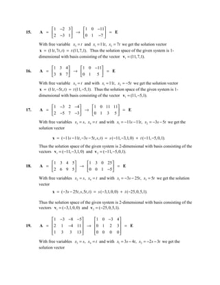3. Specific examples involve finding bases for solution spaces of systems of linear equations by reducing the coefficient matrices to echelon form and writing the general solutions in terms of the basis vectors.

1. SECTION 4.4
BASES AND DIMENSION FOR VECTOR SPACES
A basis {v1 , v 2 , , v k } for a subspace W of Rn enables up to visualize W as a k-dimensional
plane (or hyperplane) through the origin in Rn. In case W is the solution space of a
homogeneous linear system, a basis for W is a maximal linearly independent set of solutions of
the system, and every other solution is a linear combination of these particular solutions.
1. The vectors v1 and v2 are linearly independent (because neither is a scalar multiple of
the other) and therefore form a basis for R2.
2. We note that v2 = 2v1. Consequently the vectors v1 , v 2 , v 3 are linearly dependent, and
therefore do not form a basis for R3.
3. Any four vectors in R3 are linearly dependent, so the given vectors do not form a basis
for R3.
4. Any basis for R4 contains four vectors, so the given vectors v1 , v 2 , v 3 do not form a
basis for R4.
5. The three given vectors v1 , v 2 , v 3 all lie in the 2-dimensional subspace x1 = 0 of R3.
Therefore they are linearly dependent, and hence do not form a basis for R3.
6. Det ([ v1 v2 v 3 ]) = −1 ≠ 0, so the three vectors are linearly independent, and hence do
form a basis for R3.
7. Det ([ v1 v2 v 3 ]) = 1 ≠ 0, so the three vectors are linearly independent, and hence do
form a basis for R3.
8. Det ([ v1 v2 v3 v 4 ]) = 66 ≠ 0, so the four vectors are linearly independent, and hence
do form a basis for R4.
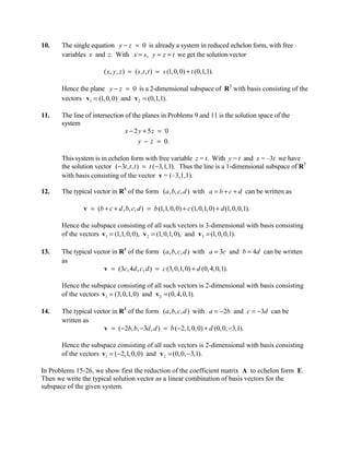
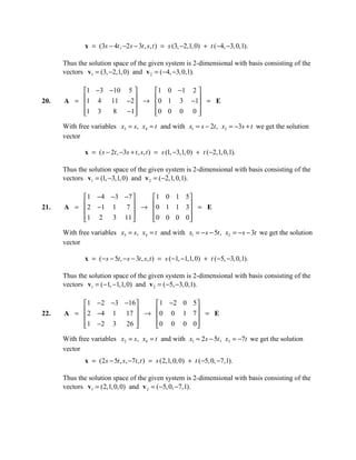
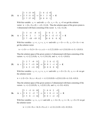
9. The single equation x − 2 y + 5 z = 0 is already a system in reduced echelon form, with
free variables y and z. With y = s, z = t , x = 2s − 5t we get the solution vector
( x, y , z ) = (2s − 5t , s, t ) = s (2,1, 0) + t (−5, 0,1).
Hence the plane x − 2 y + 5 z = 0 is a 2-dimensional subspace of R3 with basis consisting
of the vectors v1 = (2,1, 0) and v 2 = (−5, 0,1).

2. 10. The single equation y − z = 0 is already a system in reduced echelon form, with free
variables x and z. With x = s, y = z = t we get the solution vector
( x, y , z ) = (s , t , t ) = s (1, 0, 0) + t (0,1,1).
Hence the plane y − z = 0 is a 2-dimensional subspace of R3 with basis consisting of the
vectors v1 = (1, 0, 0) and v 2 = (0,1,1).
11. The line of intersection of the planes in Problems 9 and 11 is the solution space of the
system
x − 2 y + 5z = 0
y − z = 0.
This system is in echelon form with free variable z = t. With y = t and x = –3t we have
the solution vector (−3t , t , t ) = t (−3,1,1). Thus the line is a 1-dimensional subspace of R3
with basis consisting of the vector v = (–3,1,1).
12. The typical vector in R4 of the form (a, b, c, d ) with a = b + c + d can be written as
v = (b + c + d , b, c, d ) = b (1,1, 0, 0) + c (1, 0,1, 0) + d (1, 0, 0,1).
Hence the subspace consisting of all such vectors is 3-dimensional with basis consisting
of the vectors v1 = (1,1, 0, 0), v 2 = (1, 0,1,0), and v 3 = (1, 0, 0,1).
13. The typical vector in R4 of the form (a, b, c, d ) with a = 3c and b = 4d can be written
as
v = (3c, 4d , c, d ) = c (3, 0,1, 0) + d (0, 4, 0,1).
Hence the subspace consisting of all such vectors is 2-dimensional with basis consisting
of the vectors v1 = (3, 0,1, 0) and v 2 = (0, 4, 0,1).
14. The typical vector in R4 of the form (a, b, c, d ) with a = −2b and c = −3d can be
written as
v = (−2b, b, −3d , d ) = b (−2,1, 0, 0) + d (0, 0, −3,1).
Hence the subspace consisting of all such vectors is 2-dimensional with basis consisting
of the vectors v1 = (−2,1, 0, 0) and v 2 = (0, 0, −3,1).
In Problems 15-26, we show first the reduction of the coefficient matrix A to echelon form E.
Then we write the typical solution vector as a linear combination of basis vectors for the
subspace of the given system.

3. 1 −2 3 1 0 −11
15. A =   → 0 1 −7  = E
 2 −3 1  
With free variable x3 = t and x1 = 11t , x2 = 7t we get the solution vector
x = (11t , 7t , t ) = t (11, 7,1). Thus the solution space of the given system is 1-
dimensional with basis consisting of the vector v1 = (11, 7,1).
1 3 4 1 0 −11
16. A =   → 0 1 5  = E
3 8 7   
With free variable x3 = t and with x1 = 11t , x2 = −5t we get the solution vector
x = (11t , −5t , t ) = t (11, −5,1). Thus the solution space of the given system is 1-
dimensional with basis consisting of the vector v1 = (11, −5,1).
 1 −3 2 −4  1 0 11 11
17. A =   → 0 1 3 5  = E
 2 −5 7 −3  
With free variables x3 = s, x4 = t and with x1 = −11s − 11t , x2 = −3s − 5t we get the
solution vector
x = ( −11s − 11t , −3s − 5t , s, t ) = s ( −11, −3,1, 0) + t (−11, −5, 0,1).
Thus the solution space of the given system is 2-dimensional with basis consisting of the
vectors v1 = (−11, −3,1, 0) and v 2 = (−11, −5,0,1).
1 3 4 5 1 3 0 25 
18. A =   → 0 0 1 −5  = E
2 6 9 5  
With free variables x2 = s, x4 = t and with x1 = −3s − 25t , x3 = 5t we get the solution
vector
x = ( −3s − 25t , s,5t , t ) = s (−3,1, 0, 0) + t (−25, 0,5,1).
Thus the solution space of the given system is 2-dimensional with basis consisting of the
vectors v1 = (−3,1, 0, 0) and v 2 = (−25, 0,5,1).
 1 −3 −8 −5   1 0 −3 4 
19.  2 1 −4 11  → 0 1 2 3  = E
A =    
1 3 3 13 
  0 0 0 0 
 
With free variables x3 = s, x4 = t and with x1 = 3s − 4t , x2 = −2 s − 3t we get the
solution vector

4. x = (3s − 4t , −2s − 3t , s, t ) = s (3, −2,1, 0) + t ( −4, −3, 0,1).
Thus the solution space of the given system is 2-dimensional with basis consisting of the
vectors v1 = (3, −2,1, 0) and v 2 = (−4, −3, 0,1).
1 −3 −10 5   1 0 −1 2 
20. 1 4 11 −2  → 0 1 3 −1 = E
A =    
1 3
 8 −1
 0 0 0 0 
 
With free variables x3 = s, x4 = t and with x1 = s − 2t , x2 = −3s + t we get the solution
vector
x = ( s − 2t , −3s + t , s, t ) = s (1, −3,1, 0) + t (−2,1, 0,1).
Thus the solution space of the given system is 2-dimensional with basis consisting of the
vectors v1 = (1, −3,1, 0) and v 2 = (−2,1, 0,1).
 1 −4 −3 −7  1 0 1 5 
21.  2 −1 1 7  → 0 1 1 3  = E
A =    
1 2 3 11 
  0 0 0 0
 
With free variables x3 = s, x4 = t and with x1 = − s − 5t , x2 = − s − 3t we get the solution
vector
x = ( − s − 5t , − s − 3t , s, t ) = s (−1, −1,1, 0) + t ( −5, −3, 0,1).
Thus the solution space of the given system is 2-dimensional with basis consisting of the
vectors v1 = (−1, −1,1, 0) and v 2 = (−5, −3,0,1).
1 −2 −3 −16   1 −2 0 5 
22.  2 −4 1 17  → 0 0 1 7  = E
A =    
1 −2 3 26 
  0 0 0 0 
 
With free variables x2 = s, x4 = t and with x1 = 2s − 5t , x3 = −7t we get the solution
vector
x = (2s − 5t , s, −7t , t ) = s (2,1, 0, 0) + t (−5, 0, −7,1).
Thus the solution space of the given system is 2-dimensional with basis consisting of the
vectors v1 = (2,1, 0, 0) and v 2 = (−5, 0, −7,1).

5. 1 5 13 14  1 0 −2 0 
23.  2 5 11 12  → 0 1 3 0  = E
A =    
 2 7 17 19 
  0 0 0 1 
 
With free variable x3 = s and with x1 = 2s, x2 = −3s, x4 = 0 we get the solution
vector x = (2 s, −3s, s, 0) = s (2, −3,1, 0). Thus the solution space of the given system is
1-dimensional with basis consisting of the vector v1 = (2, −3,1, 0).
 1 3 −4 −8 6  1 0 2 1 3 
24. 1 0 2
A =  1  → 0 1 −2 −3 1  = E
3  
 2 7 −10 −19 13
  0 0 0 0 0 
 
With free variables x3 = r , x4 = s, x5 = t and with x1 = −2r − s − 3t , x2 = 2r + 3s − t we
get the solution vector
x = ( −2r − s − 3t , 2r + 3s − t , r , s, t ) = r (−2, 2,1, 0, 0) + s (−1,3, 0,1, 0) + t (−3, −1, 0, 0,1).
Thus the solution space of the given system is 3-dimensional with basis consisting of the
vectors v1 = (−2, 2,1, 0, 0), v 2 = (−1,3, 0,1, 0), and v 3 = (−3, −1, 0, 0,1).
1 2 7 −9 31 1 2 0 −2 3 
25.  2 4 7 −11 34  → 0 0 1 −1 4  = E
A =    
 3 6 5 −11 29 
  0 0 0 0 0 
 
With free variables x2 = r , x4 = s, x5 = t and with x1 = −2r + 2 s − 3t , x3 = s − 4t we get
the solution vector
x = ( −2r + 2 s − 3t , r , s − 4t , s, t ) = r ( −2,1, 0, 0, 0) + s (2, 0,1,1, 0) + t ( −3, 0, −4, 0,1).
Thus the solution space of the given system is 3-dimensional with basis consisting of the
vectors v1 = (−2,1, 0, 0, 0), v 2 = (2, 0,1,1, 0), and v3 = (−3, 0, −4, 0,1).
 3 1 −3 11 10  1 0 0 2 −3
26.  5 8 2 −2 7  →  0 1 0 −1 4  = E
A =    
 2 5 0 −1 14 
   0 0 1 −2 −5 
 
With free variables x4 = s, x5 = t and with x1 = −2s + 3t , x2 = s − 4t , x3 = 2s + 5t we get
the solution vector
x = ( −2s + 3t , s − 4t , 2 s + 5t , s, t ) = s ( −2,1, 2,1, 0) + t (3, −4,5, 0,1).

6. Thus the solution space of the given system is 2-dimensional with basis consisting of the
vectors v1 = (−2,1, 2,1, 0) and v 2 = (3, −4,5, 0,1).
27. If the vectors v1 , v 2 , , v n are linearly independent, and w is another vector in V, then
the vectors w, v1 , v 2 , , v n are linearly dependent (because no n+1 vectors in the n-
dimensional vector space V are linearly independent). Hence there exist scalars
c, c1 , c2 , , cn not all zero such that
cw + c1 v1 + c2 v 2 + + cn v n = 0.
If c = 0 then the coefficients c1 , c2 , , cn would not all be zero, and hence this equation
would say (contrary to hypothesis) that the vectors v1 , v 2 , , v n are linearly dependent.
Therefore c ≠ 0, so we can solve for w as a linear combination of the vectors
v1 , v 2 , , v n . Thus the linearly independent vectors v1 , v 2 , , v n span V, and
therefore form a basis for V.
28. If the n vectors in S were not linearly independent, then some one of them would be a
linear combination of the others. These remaining n–1 vectors would then span the n-
dimensional vector space V, which is impossible. Therefore the spanning set S is also
linearly independent, and therefore is a basis for V.
29. Suppose cv + c1v1 + c2 v 2 + + ck v k = 0. Then c = 0 because, otherwise, we could
solve for v as a linear combination of the vectors v1 , v 2 , , v k . But this is impossible,
because v is not in the subspace W spanned by v1 , v 2 , , v k . It follows that
c1v1 + c2 v 2 + + ck v k = 0, which implies that c1 = c2 = = ck = 0 also, because the
vectors v1 , v 2 , , v k are linearly independent. Hence we have shown that the k+1
vectors v, v1 , v 2 , , v k are linearly independent.
30. Let S = {v1 , v 2 , , v k } be a linearly independent set of k n vectors in V. If the
vector v k +1 in V is not in W = span(S), then Problem 29 implies that the k+1 vectors
v1 , v 2 , , v k , v k +1 are linearly independent. Continuing in this fashion, we can add one
vector at a time until we have n linearly independent vectors in V, which then form a
basis for V that contains the original basis S.
31. If v k +1 is a linear combination of the vectors v1 , v 2 , , v k , then obviously every linear
combination of the vectors v1 , v 2 , , v k , v k +1 is also a linear combination of
v1 , v 2 , , v k . But the former set of k+1 vectors spans V, so the latter set of k vectors
also spans V.

7. 32. If the spanning set S for V is not linearly independent, then some vector in S is a
linear combination of the others. But Problem 31 says that when we remove this
dependent vector from S, the resulting set of one fewer vectors still spans V.
Continuing in this fashion, we remove one vector at a time from S until we wind up with
a spanning set for V that is also a linearly independent set, and therefor forms a basis for
V that is contained by the original spanning set S.
33. If S is a maximal linearly independent set in V, the we see immediately that every other
vector in V is a linear combination of the vectors in S. Thus S also spans V, and is
therefore a basis for V.
34. If the minimal spanning set S for V were not linearly independent, then (by Problem
28) some vector S would be a linear combination of the others. Then the set obtained
from the minimal spanning set S by deleting this dependent vector would be a smaller
spanning set for S (which is impossible). Hence the spanning set S is also a linearly
independent set, and therefore is a basis for V.
35. Let S = {v1 , v 2 , , v n } be a uniquely spanning set for V. Then the fact, that
0 = 0 v1 + 0 v 2 + + 0 v n
is the unique expression of the zero vector 0 as a linear combination of the vectors in S,
means that S is a linearly independent set of vectors. Hence S is a basis for V.
36. If a1 , a2 , , ak are scalars, then the linear combination c1v1 + c2 v 2 + + ck v k — of the
column vectors of the matrix in Eq. (12) having the k × k identity matrix as its bottom
k × k submatrix — is a vector of the form (*, *, , *, a1 , a2 , , ak ) . Hence this linear
combination can equal the zero vector only if a1 = a2 = = ak = 0. Thus the vectors
v1 , v 2 , , v k are linearly independent.