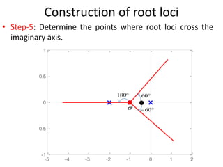
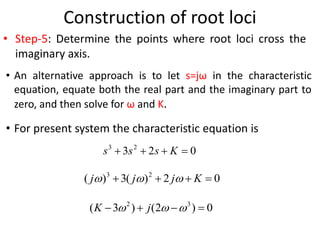
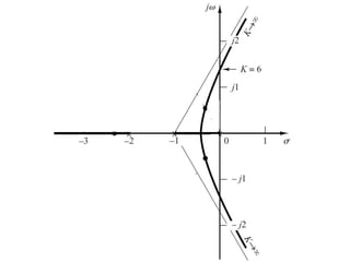
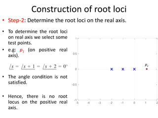
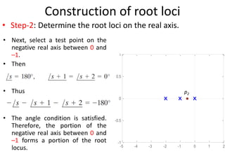
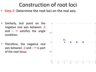
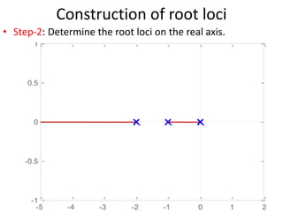
The document explains the concept of root locus, detailing its significance in control engineering as the trajectory of the roots of the characteristic equation in the s-plane as a system parameter changes. It outlines steps for constructing root loci, including locating open-loop poles and zeros, determining asymptotes, and identifying breakaway and break-in points. Additionally, it addresses the importance of angle and magnitude conditions in roots location and methods for analyzing systems to predict the effects of parameter variations.


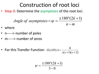
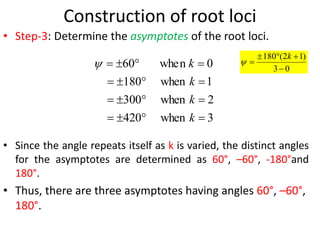


![Solution
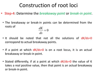
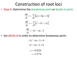
• Differentiating K with respect to s and setting the derivative equal to zero yields;
Hence, solving for s, we find the
break-away and break-in points; s = -1.45 and 3.82
1
2
3
)
15
8
(
2
2
s
s
s
s
K
)
15
8
(
)
2
3
(
2
2
s
s
s
s
K
0
)
15
8
(
)]
8
2
)(
2
3
(
)
3
2
)(
15
8
[(
2
2
2
2
s
s
s
s
s
s
s
s
ds
dK
0
61
26
11 2
s
s](https://image.slidesharecdn.com/chap8lect-240717064216-01acfd1d/85/control-Systems-for-Biomedical-lect-pptx-32-320.jpg)