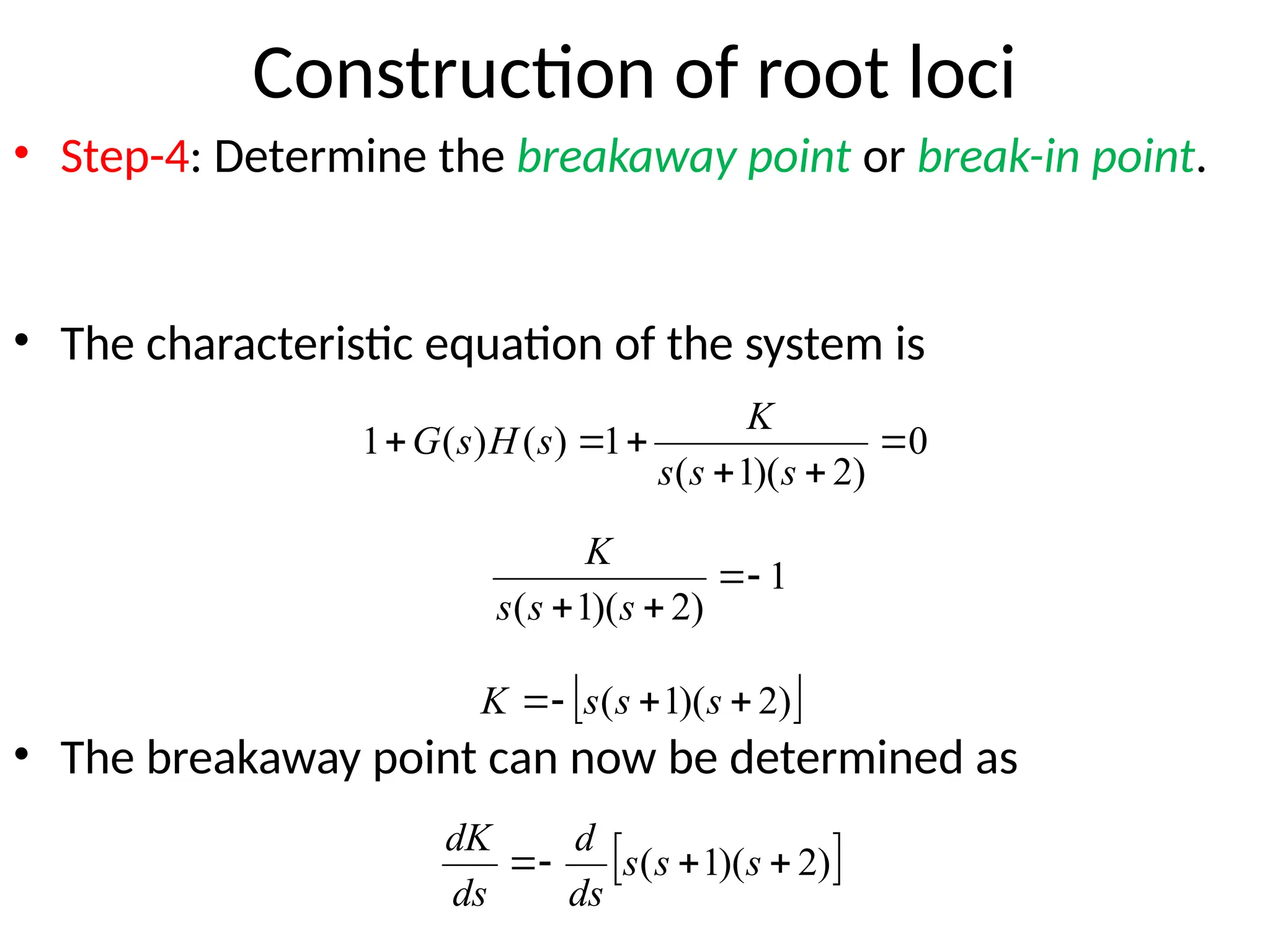
Root Locus . ppt x construction of root locii

Digital and Non-Linear Control
Root Locus

Outline
• Introduction
• Angle and Magnitude Condition
• Construction of Root Loci
• Examples

Introduction
• Consider a unity feedback control system shown
below.
• The open loop transfer function G(s) of the system
is
• And the closed transfer function is
K
s
K
s
G
s
G
s
R
s
C





1
)
(
1
)
(
)
(
)
(
1

s
K
)
(s
R )
(s
C
1
)
(


s
K
s
G

Introduction
• Location of closed loop Pole for different values of K
(remember K>0).
K
s
K
s
R
s
C



1
)
(
)
(
K Pole
0.5 -1.5
1 -2
2 -3
3 -4
5 -6
10 -11
15 -16
Pole-Zero Map
Imaginary
Axis
-16 -14 -12 -10 -8 -6 -4 -2
-0.5
0
0.5
1

What is Root Locus?
• The root locus is the path of the roots of the
characteristic equation traced out in the s-plane
as a system parameter varies from zero to infinity.

How to Sketch root locus?
• One way is to compute the roots of the
characteristic equation for all possible values
of K.
K
s
K
s
R
s
C



1
)
(
)
(
K Pole
0.5 -1.5
1 -2
2 -3
3 -4
5 -6
10 -11
15 -16

How to Sketch root locus?
• Computing the roots for all values of K might
be tedious for higher order systems.
K
s
s
s
s
K
s
R
s
C





)
20
)(
10
)(
1
(
)
(
)
(
K Pole
0.5 ?
1 ?
2 ?
3 ?
5 ?
10 ?
15 ?

Construction of Root Loci
• Finding the roots of the characteristic equation of degree
higher than 3 is laborious and will need computer solution.
• A simple method for finding the roots of the characteristic
equation has been developed by W. R. Evans and used
extensively in control engineering.
• This method, called the root-locus method, is one in which
the roots of the characteristic equation are plotted for all
values of a system parameter.

• The roots corresponding to a particular value of this
parameter can then be located on the resulting
graph.
• By using the root-locus method the designer can
predict the effects on the location of the closed-loop
poles of varying the gain value or adding open-loop
poles and/or open-loop zeros.

Angle & Magnitude Conditions
• In constructing the root loci angle and magnitude
conditions are important.
• Consider the system shown in following figure.
• The closed loop transfer function is
)
(
)
(
1
)
(
)
(
)
(
s
H
s
G
s
G
s
R
s
C



• The characteristic equation is obtained by setting the
denominator polynomial equal to zero.
• Or
• Since G(s)H(s) is a complex quantity it can be split
into angle and magnitude part.
0
)
(
)
(
1 
 s
H
s
G
1
)
(
)
( 

s
H
s
G

• The angle of G(s)H(s)=-1 is
• Where k=1,2,3…
• The magnitude of G(s)H(s)=-1 is
)
1
2
(
180
)
(
)
(
1
)
(
)
(








k
s
H
s
G
s
H
s
G

1
)
(
)
(
1
)
(
)
(



s
H
s
G
s
H
s
G

• Angle Condition
• Magnitude Condition
• The values of s that fulfill both the angle and
magnitude conditions are the roots of the
characteristic equation, or the closed-loop poles.
...)
3
,
2
,
1
(
)
1
2
(
180
)
(
)
( 



 k
k
s
H
s
G 
1
)
(
)
( 
s
H
s
G

Construction of root loci
• Step-1: The first step in constructing a root-locus plot
is to locate the open-loop poles and zeros in s-plane.
)
2
)(
1
(
)
(
)
(



s
s
s
K
s
H
s
G
-5 -4 -3 -2 -1 0 1 2
-1
-0.5
0
0.5
1
Pole-Zero Map
Real Axis
Imaginary
Axis
)
2
(
)
1
(
is
angle
The 






 s
s
s

-5 -4 -3 -2 -1 0 1 2
-1
-0.5
0
0.5
1
Pole-Zero Map
Real Axis
Imaginary
Axis
• Step-2: Determine the root loci on the real axis.
p1
• To determine the root loci
on real axis we select some
test points.
• e.g: p1 (on positive real axis).
• The angle condition is not
satisfied.
• Hence, there is no root
locus on the positive real
axis.

-5 -4 -3 -2 -1 0 1 2
-1
-0.5
0
0.5
1
Pole-Zero Map
Real Axis
Imaginary
Axis
p2
• Next, select a test point on the
negative real axis between 0 and
–1.
• Then
• Thus
• The angle condition is satisfied.
Therefore, the portion of the
negative real axis between 0 and
–1 forms a portion of the root
locus.

-5 -4 -3 -2 -1 0 1 2
-1
-0.5
0
0.5
1
Pole-Zero Map
Real Axis
Imaginary
Axis
p3
• Now, select a test point on the
negative real axis between -1 and
–2.
• Then
• Thus
• The angle condition is not
satisfied. Therefore, the negative
real axis between -1 and –2 is not
a part of the root locus.

-5 -4 -3 -2 -1 0 1 2
-1
-0.5
0
0.5
1
Pole-Zero Map
Real Axis
Imaginary
Axis
p4
• Similarly, test point on the
negative real axis between -2
and – ∞ satisfies the angle
condition.
• Therefore, the negative real
axis between -2 and – ∞ is
part of the root locus.

-5 -4 -3 -2 -1 0 1 2
-1
-0.5
0
0.5
1
Pole-Zero Map
Imaginary
Axis

• Step-3: Determine the asymptotes of the root loci. That is, the
root loci when s is far away from origin.
Asymptote is the straight line approximation of a curve
Actual Curve
Asymptotic Approximation
𝜎
Ψ

• Step-3: Determine the asymptotes of the root loci.
• where
• n-----> number of poles
• m-----> number of zeros
• For this Transfer Function
m
n
k
asymptotes
of
Angle






)
1
2
(
180

)
2
)(
1
(
)
(
)
(



s
s
s
K
s
H
s
G
0
3
)
1
2
(
180





k


• Since the angle repeats itself as k is varied, the distinct angles
for the asymptotes are determined as 60°, –60°, and 180°.
3
when
420
2
when
300
1
when
180
0
n
whe
60
















k
k
k
k
 0
3
)
1
2
(
180





k


• Before we can draw these asymptotes in the complex
plane, we need to find the point where they intersect the
real axis.
• Point of intersection of asymptotes on real axis (or
centroid of asymptotes) is
m
n
zeros
poles







• For
0
3
0
)
2
1
0
(






)
2
)(
1
(
)
(
)
(



s
s
s
K
s
H
s
G
1
3
3






-5 -4 -3 -2 -1 0 1 2
-1
-0.5
0
0.5
1
Pole-Zero Map
Real Axis
Imaginary
Axis


60

 60

180




 180
,
60
,
60

1




• Step-4: Determine the breakaway/break-in point.
• The breakaway/break-in
point is the point from
which the root locus
branches leaves/arrives
real axis.
-5 -4 -3 -2 -1 0 1 2
-1
-0.5
0
0.5
1
Pole-Zero Map
Real Axis
Imaginary
Axis

• Step-4: Determine the breakaway point or break-in point.
• The breakaway or break-in points can be determined from the
roots of (page 275)
• It should be noted that not all the solutions of dK/ds=0
correspond to actual breakaway points.
• If a point at which dK/ds=0 is on a root locus, it is an actual
breakaway or break-in point.
0

ds
dK

• The characteristic equation of the system is
• The breakaway point can now be determined as
0
)
2
)(
1
(
1
)
(
)
(
1 





s
s
s
K
s
H
s
G
1
)
2
)(
1
(



 s
s
s
K
 
)
2
)(
1
( 


 s
s
s
K
 
)
2
)(
1
( 


 s
s
s
ds
d
ds
dK

• Set dK/ds=0 in order to determine breakaway point.
 
)
2
)(
1
( 


 s
s
s
ds
d
ds
dK
 
s
s
s
ds
d
ds
dK
2
3 2
3




2
6
3 2



 s
s
ds
dK
0
2
6
3 2



 s
s
0
2
6
3 2


 s
s
5774
.
1
4226
.
0




s

• Since the breakaway point needs to be on a root locus
between 0 and –1, it is clear that s=–0.4226 corresponds to
the actual breakaway point.
• Point s=–1.5774 is not on the root locus. Hence, this point is
not an actual breakaway or break-in point.
5774
.
1
4226
.
0




s
)
2
)(
1
(
)
(
)
(



s
s
s
K
s
H
s
G

• Step-4: Determine the breakaway point.
-5 -4 -3 -2 -1 0 1 2
-1
-0.5
0
0.5
1
Pole-Zero Map
Real Axis
Imaginary
Axis


60

 60

180
4226
.
0


s

• Step-4: Determine the breakaway point.
4226
.
0


s
-5 -4 -3 -2 -1 0 1 2
-1
-0.5
0
0.5
1
Pole-Zero Map
Real Axis
Imaginary
Axis

• Step-5: Determine the points where root loci cross the
imaginary axis.
-5 -4 -3 -2 -1 0 1 2
-1
-0.5
0
0.5
1
Pole-Zero Map
Imaginary
Axis


60

 60

180

imaginary axis.
• Let s=jω in the characteristic equation, equate both the real
part and the imaginary part to zero, and then solve for ω and
K.
• For present system the characteristic equation is
0
2
3 2
3



 K
s
s
s
0
2
)
(
3
)
( 2
3



 K
j
j
j 


0
)
2
(
)
3
( 3
2



 

 j
K

imaginary axis.
• Equating both real and imaginary parts of this equation
to zero
• Which yields
0
)
2
(
)
3
( 3
2



 

 j
K
0
)
3
( 2

 
K
0
)
2
( 3

 


-7 -6 -5 -4 -3 -2 -1 0 1 2
-5
-4
-3
-2
-1
0
1
2
3
4
5
Root Locus
Real Axis
Imaginary
Axis

Example
• Determine the Breakaway and breakin points

Solution
• Differentiating K with respect to s and setting the derivative equal to zero yields;
Hence, solving for s, we find the
break-away and break-in points s = -1.45 and 3.82
1
2
3
)
15
8
(
2
2






s
s
s
s
K
)
15
8
(
)
2
3
(
2
2






s
s
s
s
K
0
)
15
8
(
)]
8
2
)(
2
3
(
)
3
2
)(
15
8
[(
2
2
2
2












s
s
s
s
s
s
s
s
ds
dK
0
61
26
11 2


 s
s
180
0
0
180
0
)
2
(
)
1
(
)
5
(
)
3
(
,
82
.
3
540
0
180
180
180
)
2
(
)
1
(
)
5
(
)
3
(
,
45
.
1






































s
s
s
s
s
s
s
s
s
s

Root Loci by MATLAB
• Example 6-4 in page 293

Root Locus . ppt x construction of root locii

More Related Content

Similar to Root Locus . ppt x construction of root locii

More from RDTCPOLYTECHNICMECHD

Recently uploaded

Root Locus . ppt x construction of root locii