Download as PDF, PPTX


![Braitenberg Vehicles: Simulink Model
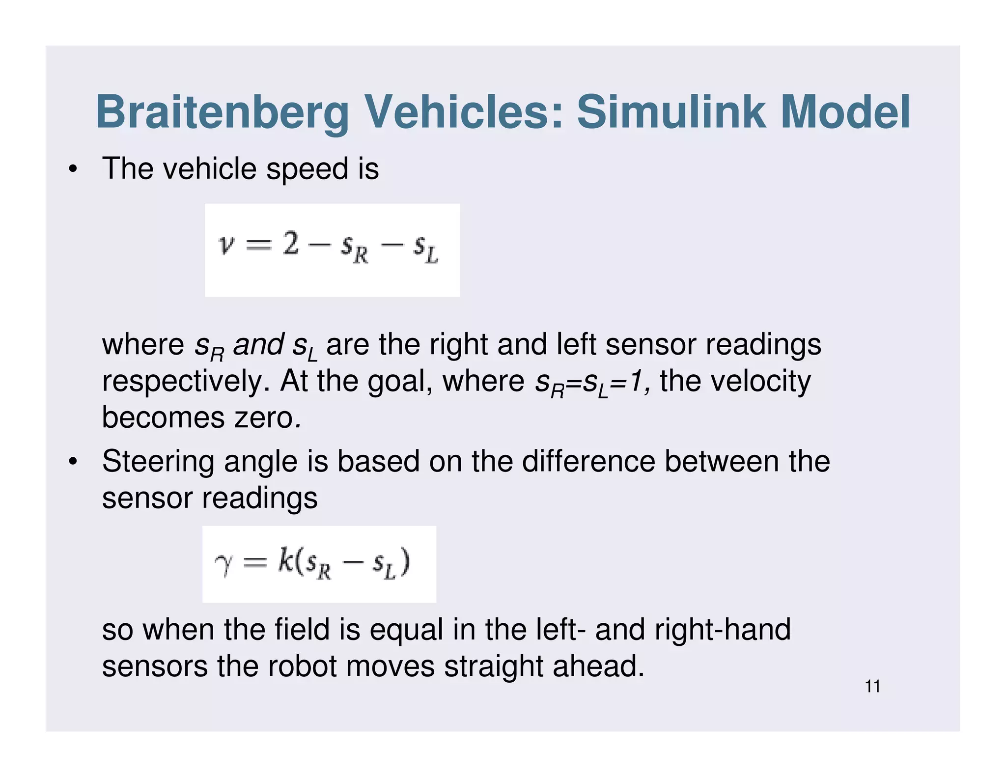
• The field to be sensed is a simple inverse square field
defined by
∈which returns the sensor value s(x, y) ∈ [0, 1] which is a
function of the sensor’s position in the plane. This
particular function has a peak value at the point (60, 90).
10](https://image.slidesharecdn.com/robotics-bme-06-s17-200829163813/75/Robotics-Navigation-10-2048.jpg)


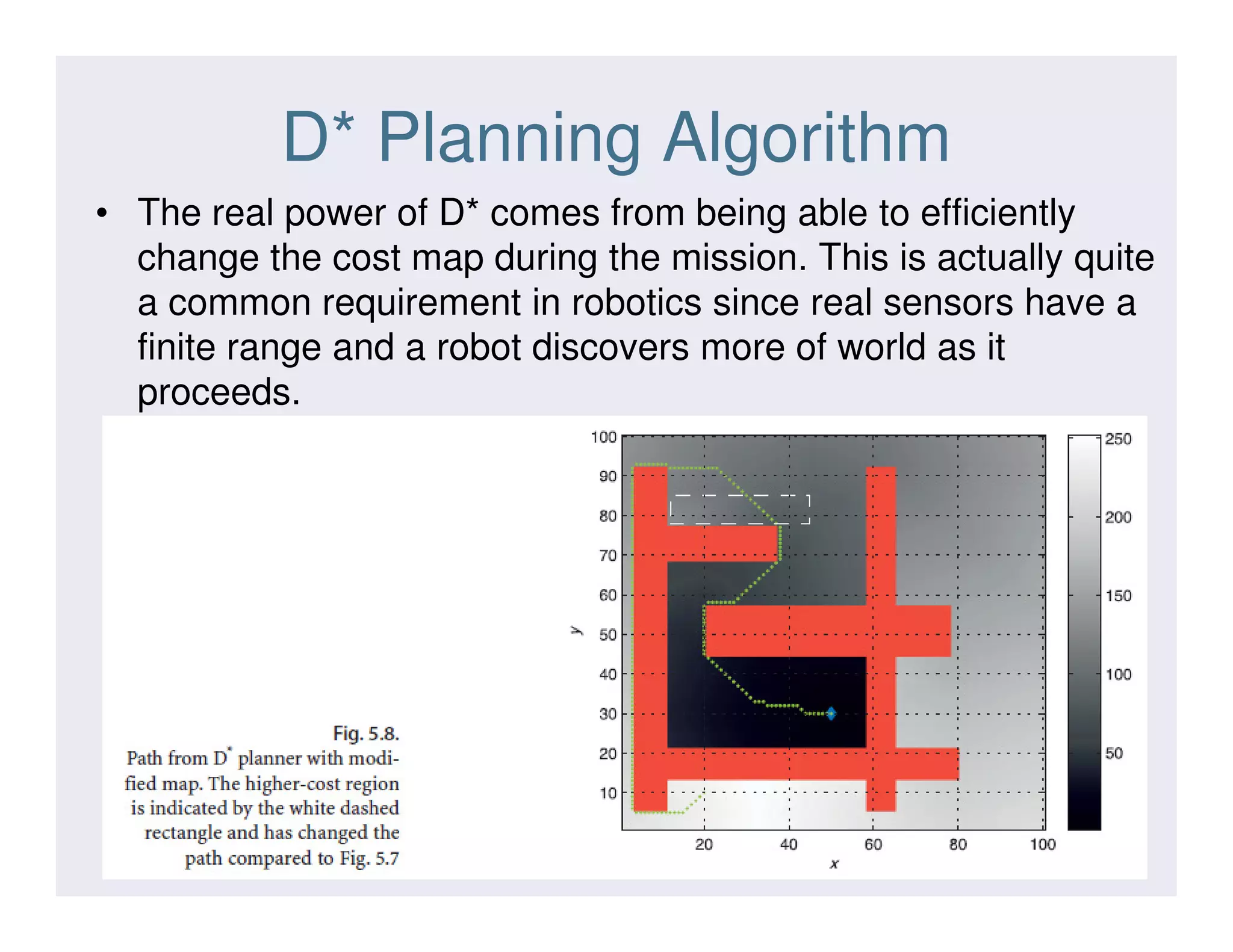


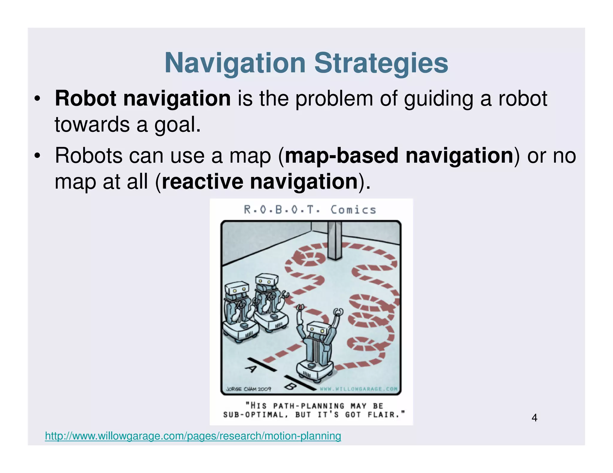
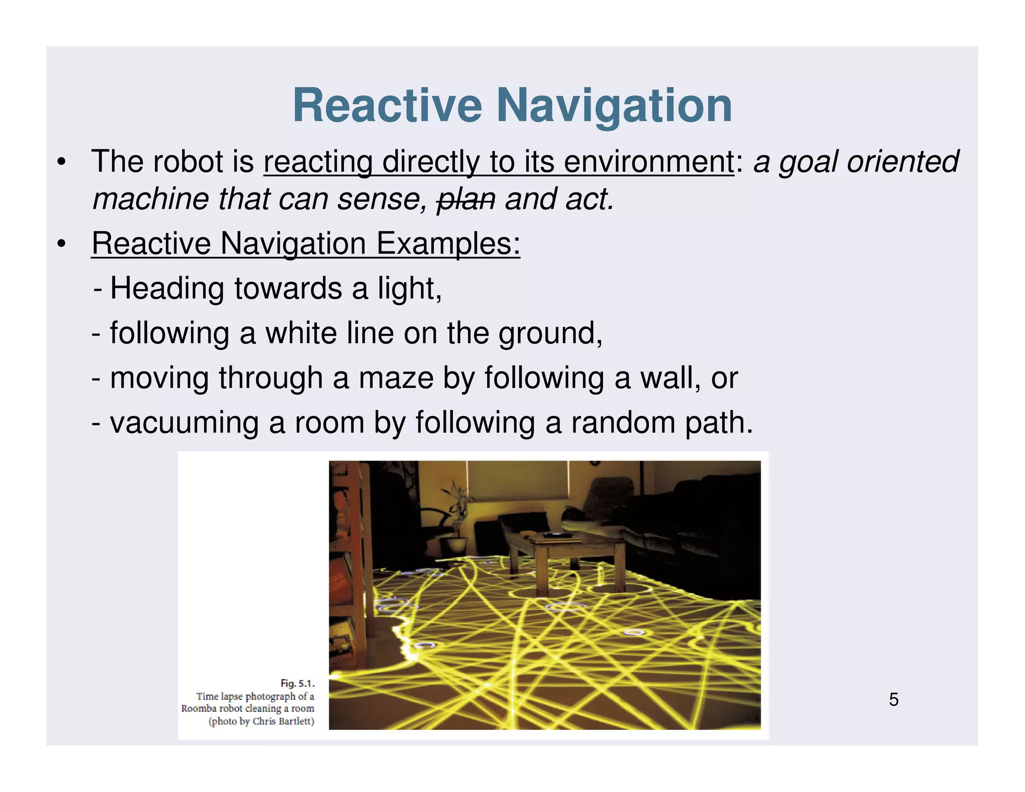
This document discusses various strategies for robot navigation, including reactive navigation using Braitenberg vehicles and simple automata, as well as map-based planning algorithms. Reactive navigation relies on direct sensor-motor connections to navigate without an internal world model, while map-based planning uses a map representation and algorithms like the distance transform or D* to find optimal paths between points. The document provides examples and explanations of different navigation techniques.