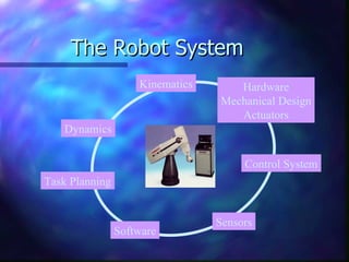
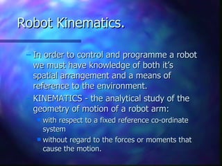
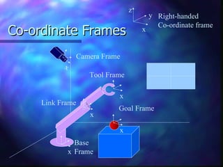
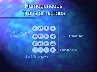
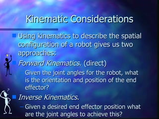
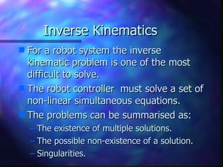
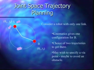
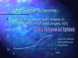
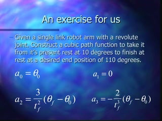
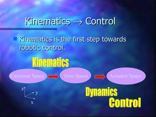
The document discusses robot kinematics and control. It covers topics like coordinate frames, homogeneous transformations, forward and inverse kinematics, joint space trajectories, and cubic polynomial path planning. Specifically: 1) Kinematics is the study of robot motion without regard to forces or moments. It describes the spatial configuration using coordinate frames and homogeneous transformations. 2) Forward kinematics determines end effector position from joint angles. Inverse kinematics determines joint angles for a desired end effector position. 3) Joint space trajectories plan motion by describing joint angle profiles over time using functions like cubic polynomials and splines. 4) Cubic polynomials satisfy constraints like initial/final position and velocity to generate smooth motion profiles for a single revol

1. The Robot System Control System Sensors Kinematics Dynamics Task Planning Software Hardware Mechanical Design Actuators

2. Robot Kinematics. In order to control and programme a robot we must have knowledge of both it’s spatial arrangement and a means of reference to the environment. KINEMATICS - the analytical study of the geometry of motion of a robot arm: with respect to a fixed reference co-ordinate system without regard to the forces or moments that cause the motion.

3. Co-ordinate Frames z y x Right-handed Co-ordinate frame x Base Frame x Tool Frame x Goal Frame x Link Frame x Camera Frame

4. Kinematic Relationship Between two frames we have a kinematic relationship - basically a translation and a rotation. This relationship is mathematically represented by a 4  4 Homogeneous Transformation Matrix. z y x z y x

5. Homogeneous Transformations  x  y 3  1 Translation  z 1 Global Scale r1 r2 r3 r4 r5 r6 r7 r8 r9 3  3 Rotational Matrix 0 0 0 1  3 Perspective

6. Kinematic Considerations Using kinematics to describe the spatial configuration of a robot gives us two approaches: Forward Kinematics . (direct) Given the joint angles for the robot, what is the orientation and position of the end effector? Inverse Kinematics . Given a desired end effector position what are the joint angles to achieve this?

7. Inverse Kinematics For a robot system the inverse kinematic problem is one of the most difficult to solve. The robot controller must solve a set of non-linear simultaneous equations. The problems can be summarised as: The existence of multiple solutions. The possible non-existence of a solution. Singularities.

8. Multiple Solutions Goal This two link planar manipulator has two possible solutions. This problem gets worse with more ‘Degrees of Freedom’. Redundancy of movement.

9. Non Existence of Solution A goal outside the workspace of the robot has no solution. An unreachable point can also be within the workspace of the manipulator - physical constraints. A singularity is a place of  acceleration - trajectory tracking. Goal

10. Kinematics  Control Kinematics is the first step towards robotic control. Cartesian Space Joint Space Actuator Space Kinematics Dynamics Control z y x

11. Joint Space Trajectories For a robot to operate efficiently it must be able to move from point to point in space. A trajectory is a time history of position, velocity and acceleration for each joint. Trajectories are computed at run time and updated at a certain rate - the Path Update Rate. (PUMA robot updates at 36Hz)

12. Joint Space Trajectory Planning Consider a robot with only one link. A B (  0 , t 0 ) (  f , t f ) Kinematics gives one configuration for B. Choice of two trajectories to get there. May wish to specify a via point - maybe to avoid an obstacle.

13. Joint Space Schemes. We need to describe path shapes in terms of functions of joint angles.  (t) angle  f time 0 t f  0 Lots of choices for continuous functions Cubic Polynomial Splines

14. Cubic Polynomials To move a single revolute joint from A to B in a given time gives four constraints. A starts at rest and at angle   B finishes at rest and at angle  f A cubic polynomial has four co-efficients which satisfy the four constraints:

15. An Exercise for you: Place the initial constraints into the formulae for position, velocity and acceleration and prove that the co-effecients are:

16. An exercise for us Given a single link robot arm with a revolute joint. Construct a cubic path function to take it from it’s present rest at 10 degrees to finish at rest at a desired end position of 110 degrees.

17. Making A Spline. A via point gives a constraint with angle time A B Via points t via1 t via2

18. More Joint Space Schemes Quintic Polynomials. The cubic polynomial does not specify accelerations at the start and end of the motion. This adds two more constraints which can only be represented by a quintic polynomial. i.e. a 5 t 5 Linear Functions with parabolic Blends. Linear function requires an infinite acceleration to get it started so parabolic blends are added at each end of the trajectory.

19. Kinematics  Control Kinematics is the first step towards robotic control. Cartesian Space Joint Space Actuator Space Kinematics Dynamics Control z y x