Motion Planning

1Guest Lecture, ECE 486: S2016 - University of Waterloo © Dr. Alaa Khamis
Motion Planning
S2016 ECE 486: Robot Dynamics and Control
Guest Lecturer: Alaa Khamis, PhD, SMIEEE
Robotics and AI Consultant at MIO, Inc., InnoVision Systems and Sypron
Smart Mobility Group Coordinator in CPAMI at University of Waterloo
Associate Professor at Suez University and Adjunct Professor at Nile University, Egypt
http://www.alaakhamis.org/
Monday June 13 and Friday June 17, 2016

MUSES_SECRET: ORF-RE Project - © PAMI Research Group – University of Waterloo
Objectives
When you have finished this lecture you should be able to:
• Recognize what a motion plan is, what it is supposed to
achieve, requirements of a path planner, how to represent a
plan, how to measure the quality of a plan and different
planning algorithms available.
• Understand different motion planning solvers such as
discrete planning, combinatorial planning, potential field
methods and sampling-based motion planning.
• Familiarize yourself with joint-space and Cartesian-space
trajectory Planning of robot manipulators.

Friday
Lecture
Monday
Lecture
• Introductory Concepts
• Motion Planning Solvers
 Discrete Planning
 Combinatorial Planning
 Sampling-based Motion Planning
 Potential Field Method
• Trajectory Planning of Robot Manipulators
 Basics of Trajectory Planning
 Joint-Space Trajectory Planning
 Cartesian-Space Trajectories
Outline

Outline

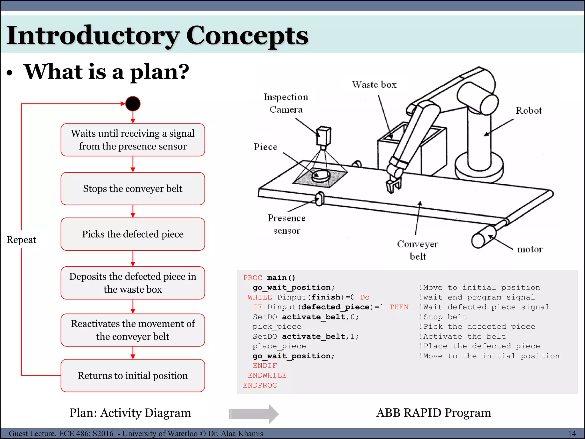
• Q: How can I get there from here?
A: Planning
Introductory Concepts
Topic
High-level Functions
Partially understood
Not fully localized
Low-level Functions
Fully understood
Localized
Perception
Situation awareness
Natural Language Understanding
Pattern Discovery
Reasoning
Decision Making
Planning
Learning
etc.
SmellHearing Taste TouchSight
Brain functions
[1]

• Planning
Planning is a complex activity that determines a future course
of actions/activities for an executing entity to drives it from
an initial state to a specified goal state. Planning often
involves reasoning with incomplete information.

• Planning is everywhere
AI Discrete Planning [2]
Piano Mover Problem [2] Unmanned Vehicles (UXVs) Planning
Rubik’s cube Sliding Puzzle
Robot Manipulator Planning
Unmanned
Aerial Vehicles
(UAV) & Micro
Aerial Vehicles
(MAV)
Unmanned
Underwater
Vehicles
(UUV)
Unmanned
Surface
Vehicles
(USV)
Unmanned
Ground
Vehicles
(UGV)

• Motion Planning
A robot has to compute a collision-free path from a start
position (s) to a given goal position (G), amidst a collection of
obstacles.
Articulated Robot Rigid Robot

Planning Entity
Planned Entity/
Execution Entity
Plan Monitoring
Plan adaptation
(Plan repair/Re-planning)
Track
Plan
Planning Environment
Mapped
Environment/
Domain Model
Planning Method/Solver
Environment Perception
• Planning Overview

• Planning Overview: Planning Environment
Different planning approaches for different environments.
Modeling Dimensions:
 Structure: structured versus unstructured.
 Observerability: fully versus partially observable.
 Determinism: deterministic versus stochastic.
 Continuity: discrete versus continuous.
 Adversary: benign versus adversarial.
 Number of agents: single agent versus multiagent.
 …

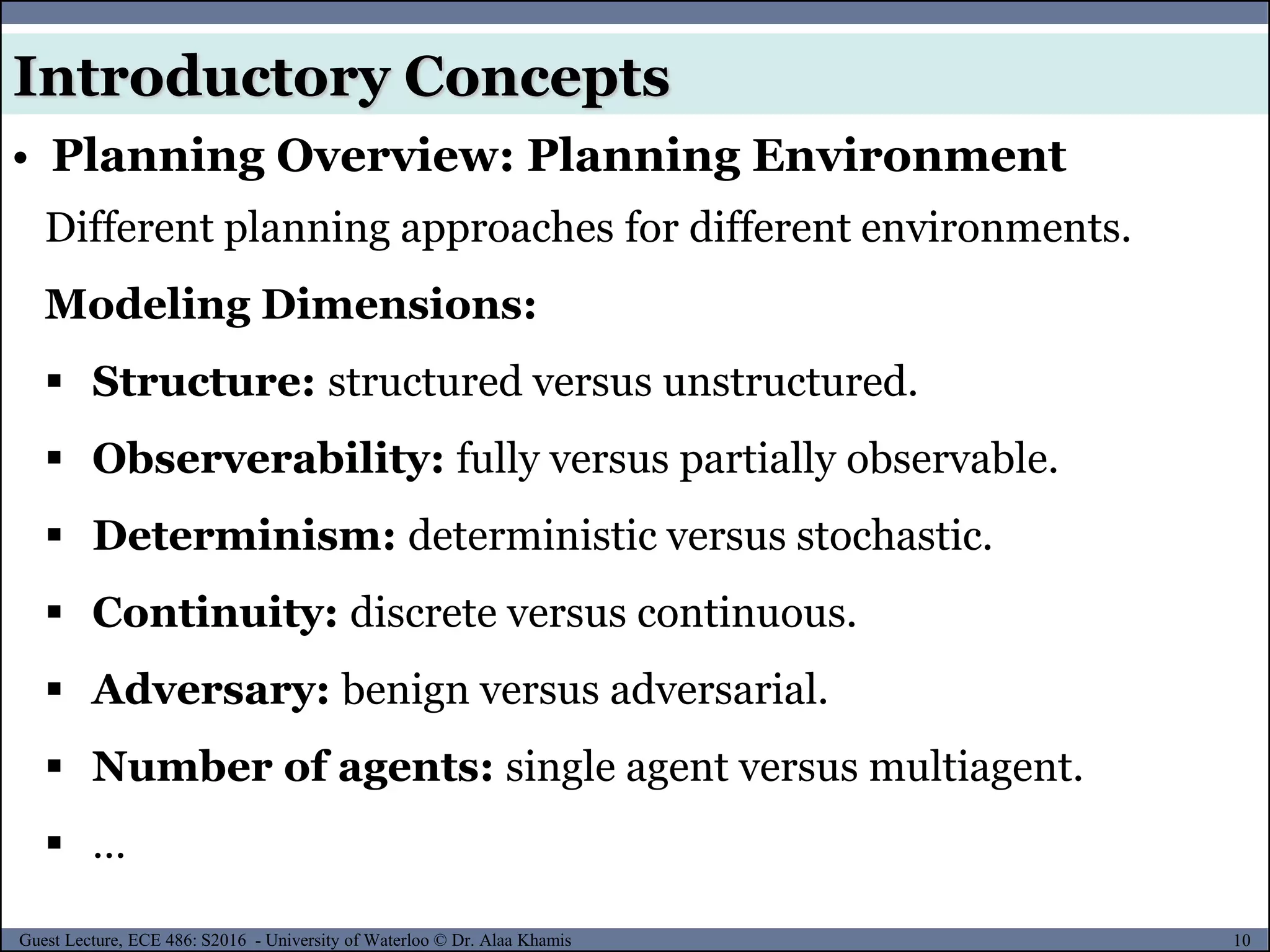
• Planning Overview: Planning Environment
Kinds of events that trigger planning [3]:
 Time-based: for example, a plan for automated
guided vehicle (AGV) needs to be made each season.
 Event-based: a plan for AGV must be made after an event,
for example, a rush order in a factory.
 Disturbance-based: a
plan must be adjusted
because a disturbance
occurs that renders the
plan invalid- for example,
unexpected moving
obstacle in the robot way. For reading: Can You Program Ethics Into a Self-Driving Car?

Domain Model
Model
Transformation
Solver Plan
• Initial state
• Goal state
• Possible states of the
robot(s)
• Primitive actions or
activities
• Hard and soft constraints
• Uncertainty (sensor and
actuators)
• A priori knowledge
• C-Space configuration
• Graph Decomposition
• Cell decomposition
• Road maps
• Potential fields
• …
• Discrete Planning
• Combinatorial Planning
• Sampling-based
Planning
• Potential Field Method
• Metaheuristics
• Planning under
Uncertainty
• Hybrid approaches
• …
• Planning Process

• Natural Questions:
◊ What is a plan?
◊ What is plan supposed to achieve?
◊ What are the requirements of a path planner?
◊ How is an environment transformed?
◊ How will plan quality be evaluated?
◊ Who or what is going to use the plan?
◊ What are the different planning algorithms?

• What is a plan?
Waits until receiving a signal
from the presence sensor
Stops the conveyer belt
Picks the defected piece
Deposits the defected piece in
the waste box
Reactivates the movement of
the conveyer belt
Returns to initial position
Repeat
Plan: Activity Diagram
PROC main()
go_wait_position; !Move to initial position
WHILE Dinput(finish)=0 Do !wait end program signal
IF Dinput(defected_piece)=1 THEN !Wait defected piece signal
SetDO activate_belt,0; !Stop belt
pick_piece !Pick the defected piece
SetDO activate_belt,1; !Activate the belt
place_piece !Place the defected piece
go_wait_position; !Move to the initial position
ENDIF
ENDWHILE
ENDPROC
ABB RAPID Program

• What is a plan?
◊ Suppose that we have a tiny mobile
robot that can move along the floor in a
building.
◊ The task is to determine a path that it
should follow from a starting location to
a goal location, while avoiding
collisions.
◊ A reasonable model can be formulated by
assuming that the robot is a moving
point in a two-dimensional
environment that contains obstacles.

• What is a plan?
◊ The task is to design an algorithm that
accepts an obstacle region defined by a
set of polygons, an initial position, and
a goal position.
◊ The algorithm must return a path that
will bring the robot from the initial
position to the goal position, while
only traversing the free space.

• What is plan supposed to achieve?
◊ A plan might simply specify a sequence of actions to be
taken; however, it may be more complicated.
◊ If it is impossible to predict future states, the plan may
provide actions as a function of state.
◊ In this case, regardless of future states, the appropriate
action is determined.
◊ It might even be the case that the state cannot be
measured.
◊ In this case, the action must be chosen based on whatever
information is available up to the current time.

• What are the requirements of a path planner?
1. to find a path through a mapped environment so that the
robot can travel along it without colliding with anything,
2.to handle uncertainty in the sensed world model and
errors in path execution,
3.to minimize the impact of objects on the field of view of the
robot’s sensors by keeping the robot away from those
objects,
4.to find the optimum path, if that path is to be negotiated
regularly.

• What are the requirements of a path planner?
5. Determine the following:
◊ Horizon: What time/space span does the
plan cover? Receding Horizon Control/planning (RHC)
◊ Frequency: How often is the plan created
or adapted?
[3]
◊ Level of detail: Does the plan need more detail in order to
be executed? Does the executing entity have to fill in the
details, or the plan used as a template for another planner
(multiresolutional planning)?
◊ (Re)presentation: How is the plan represented and
depicted? Does it specify the end state, or does it provide a
process description that leads to the end state?

• How is an environment transformed?
◊ The first step of any path-planning system is to transform
the continuous environmental model into a discrete
map suitable for the chosen path-planning algorithm.
◊ Path planners differ as to how they effect this discrete
decomposition.
R
SE
S
S
SES ES NE
……… …
Graph
Decomposition:
Environment is
represented as an
ordered directed
graph.

Cell decomposition: discriminate between
free and occupied cells.

Road map: identify a set of
routes within the free space.
Potential field: impose a mathematical
function over the space.

◊ Configuration space (C-Space) is the set of legal
configurations of the robot.
◊ C-Space also defines the topology of continuous motions.
Transform.
• Configuration space
Source: https://www.youtube.com/watch?v=zLEIWt6XZDY

For both articulated
robots and rigid-object
robots (no joints)
there exists a
transformation to the
robot and obstacles
that turns the robot
into a single point.
The C-Space
Transform.
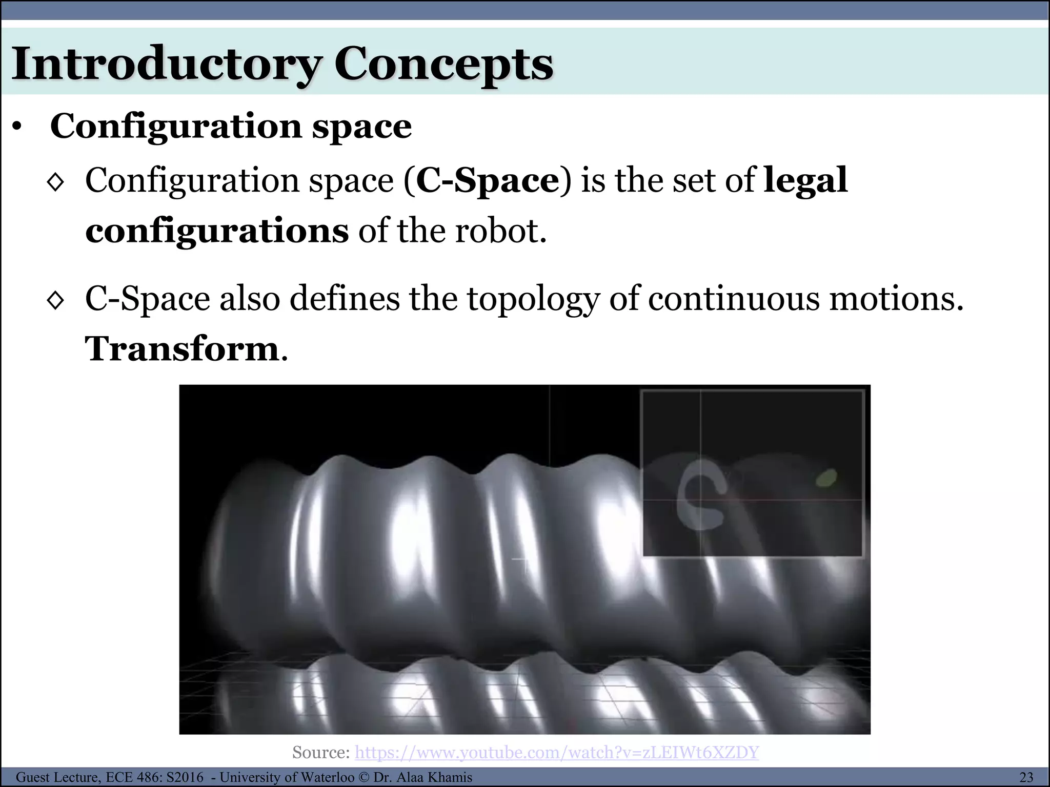
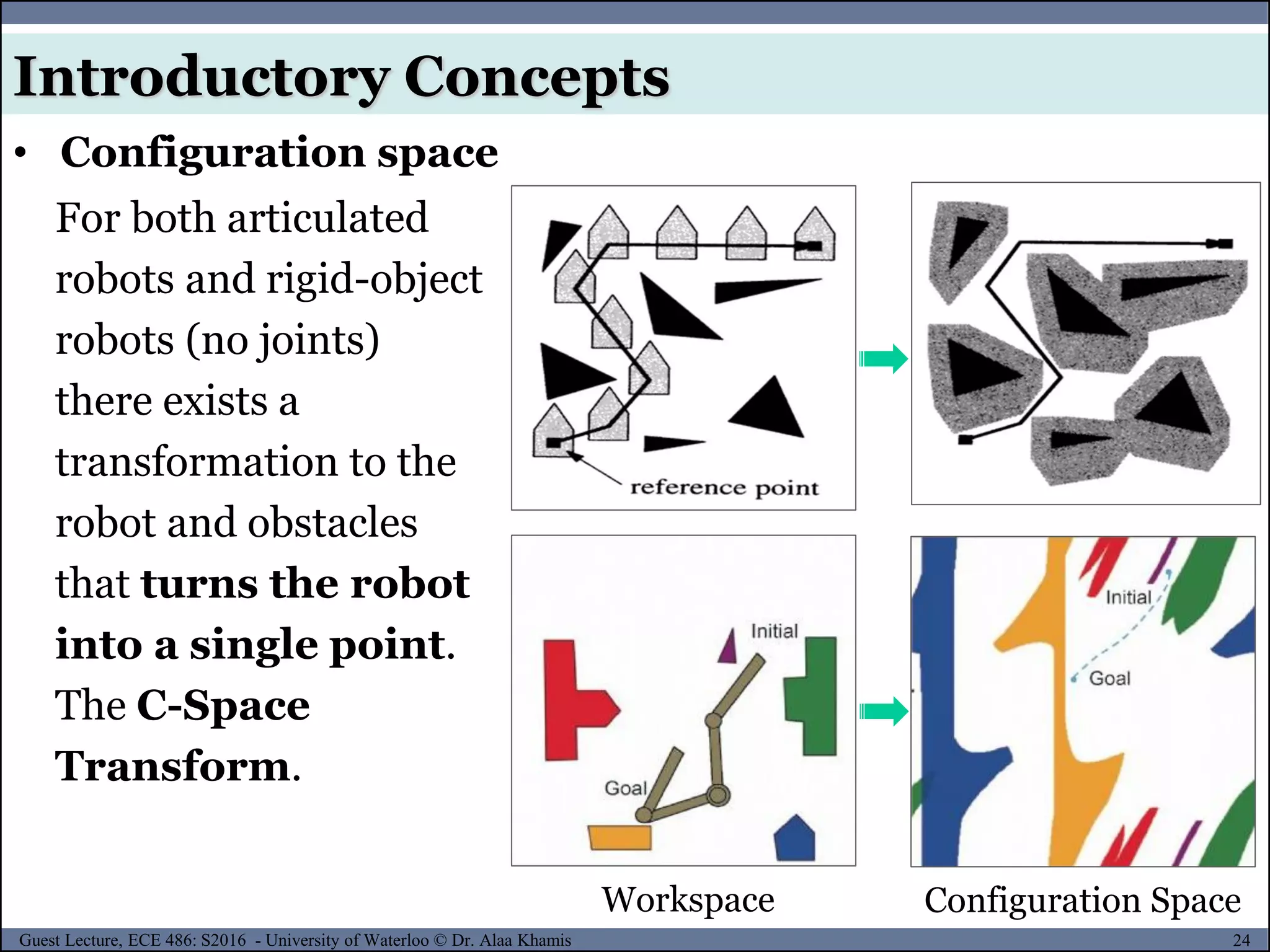
Workspace Configuration Space

Assume the following:
[4]
𝒜 : a rigid/articulated robot;
𝒲 : the workspace (i.e., the Cartesian
space in which the robot moves);
𝒜(𝑞) : the subset of the workspace that is
occupied by the robot at configuration q
𝒪𝑖 : the obstacles in the workspace;
𝒪 = ⋃𝒪𝑖, obstructive region and
𝒞 : configuration space, which is the set of all possible
configurations. A complete specification of the location of every
point on the robot is referred to as a configuration.

[4]
𝒞obs: configuration space obstacle,
which is the set of configurations for
which the robot collides with an
obstacle, 𝒞obs ⊆ 𝒞
The set of collision-free configurations, referred to as the free
configuration space, is then simply
𝒞free = 𝒞𝒞obs
𝒞obs = 𝑞 ∈ 𝒞|𝒜(𝑞)⋂𝒪 ≠ 𝜙
𝒞 = 𝒞free ∪ 𝒞obs

[4]
The path planning problem is to find a
path from an initial configuration qinit to a
final configuration qfinal, such that the robot
does not collide with any obstacle as it
traverses the path.
A collision-free path from qinit to qfinal is a continuous map,
𝒯: 0,1 → 𝒞free
with
𝒯(0)= qinit and
𝒯(1)= qfinal
qinit
qfinal
𝒞free
𝒞obs

• Configuration space: Articulated Robots
Consider a two-link planar arm in a workspace containing a
single obstacle
Two-link Planar Arm Configuration Space
[4]
The region 𝒞obswas computed
using a discrete grid on the
configuration space
Collision-free cells
Obstructive
cells

Free Space
Robot
(treat as point object)x,y
ObstaclesFree Space
Robot
x,y
• Configuration space: Rigid Robots
Workspace Configuration Space

• C-Space Transform Examples
…is equivalent to…
Where can I move this robot
in the vicinity of this obstacle
Where can I move this point in the
vicinity of this expanded obstacle
Where can I move this robot
in the vicinity of this obstacle
Where can I move this point in the
vicinity of this expanded obstacle
…is equivalent to…
Assuming you’re not
allowed to rotate

• Object-growth Algorithm
1. Attach a coordinate frame to the reference point,
2. Flip the robot about the two axes of the coordinate frame, one axis at
a time.
3. Place the reference point of the flipped robot at each of the vertices
of the object and calculate the positions of the vertices of the robot.
4. Find the convex hull of the vertices. The convex hull is the convex
polygon formed by stretching a rubber band around the vertices.

1. Attach a coordinate frame to the reference point,
2. Flip the robot about the two axes of the coordinate frame, one axis at a
time.

3. Place the reference point of the flipped robot at each of the vertices of
the object and calculate the positions of the vertices of the robot.
4. Find the convex hull of the vertices. The convex hull is the convex
polygon formed by stretching a rubber band around the vertices.
Flipped robot

• Convex hull Algorithm: Sklansky’s Algorithm
1. Place vertices into a counter-clockwise ordered list
2. Allocate a stack
3. Push vertex 0 onto stack
4. Push vertex 1 onto stack
5. For i=2 to n do
{compare vertex i to ray formed by the 2 vertices at the top of the stack}
if vertex i is on or to the right of the ray (stacktop-1, stacktop) then
pop {discard top element of stack}
End
push vertex i {put vertex i onto stack}
End
Stack (LIFO)

• Convex hull Algorithm: Sklansky’s Algorithm
Point Pushed Popped Stack
0 0 - 0
1 1 - 1,0
2
3
4
5
6
7
8
9
… … … …
Repeat…
2 1 2,0
3 2 3,0
4 - 4,3,0
5 4 5,3,0
6 5 6,3,0
7 6 7,3,0
8 - 8,7,3,0
8 9,7,3,0

• How will plan quality be evaluated?
Introductory ConceptsEvaluationMetrics
Expense
Distance from obstacles
Smoothness of the path
Time
Distance travelled
Optimality of the path
etc…

• Who or what is going to use the plan?
global
local
Raw data
Environment Model
Local Map
“Position”
Global Map
Actuator Commands
Sensing Acting
Information
Extraction
Path
Execution
Cognition
Path Planning
Knowledge,
Data Base
Mission
Commands
Path
Real World
Environment
Localization
Map Building
MotionControl
Perception
[5]

Motion Planning Methods
Discrete
Planning
• What are the different planning algorithms?
Forward
Search
Backward
Search
◊ Breadth first
◊ Depth first
◊ Dijkstra’s
algorithm
◊ A*
◊ …
Combinatorial
Planning
Cell
Decomposition
Roadmaps
◊ Voronoi Diagrams
◊ Visibility Graph
◊ Free Way Net
◊ Silhouette
◊ MAKLINK
◊ …
◊ Exact
◊ Approximate
(Fixed/
Adaptive)
Other
Approaches
◊ Sampling-Based
Motion Planning
(Rapidly-exploring
Random Trees-RRTs,
Probabilistic
Roadmaps-PRMs)
◊ Potential Field
Methods
◊ Metaheuristics
◊ Decision-theoretic
Planning
◊ Hybrid approaches

Outline

• The typical approach towards the problem of path planning
assumes a graph representation of the terrain. The problem
of minimum-path planning on a graph is well known, and a
variety of algorithms are applicable under different input
specification.
• Therefore path planning problem is handled as a search
problem to find the shortest path between start and goal
points on a graph.
Discrete Planning

Forward Graph Search Methods/
Enumerative Algorithms
Informed SearchUninformed/Blind Search
◊ Breadth-first (BFS)
◊ Depth-first (DFS)
◊ British Museum Search
or Brute-force Search
◊ Dijkstra
◊ …
◊ Best-first
◊ A*
◊ …
Discrete Planning

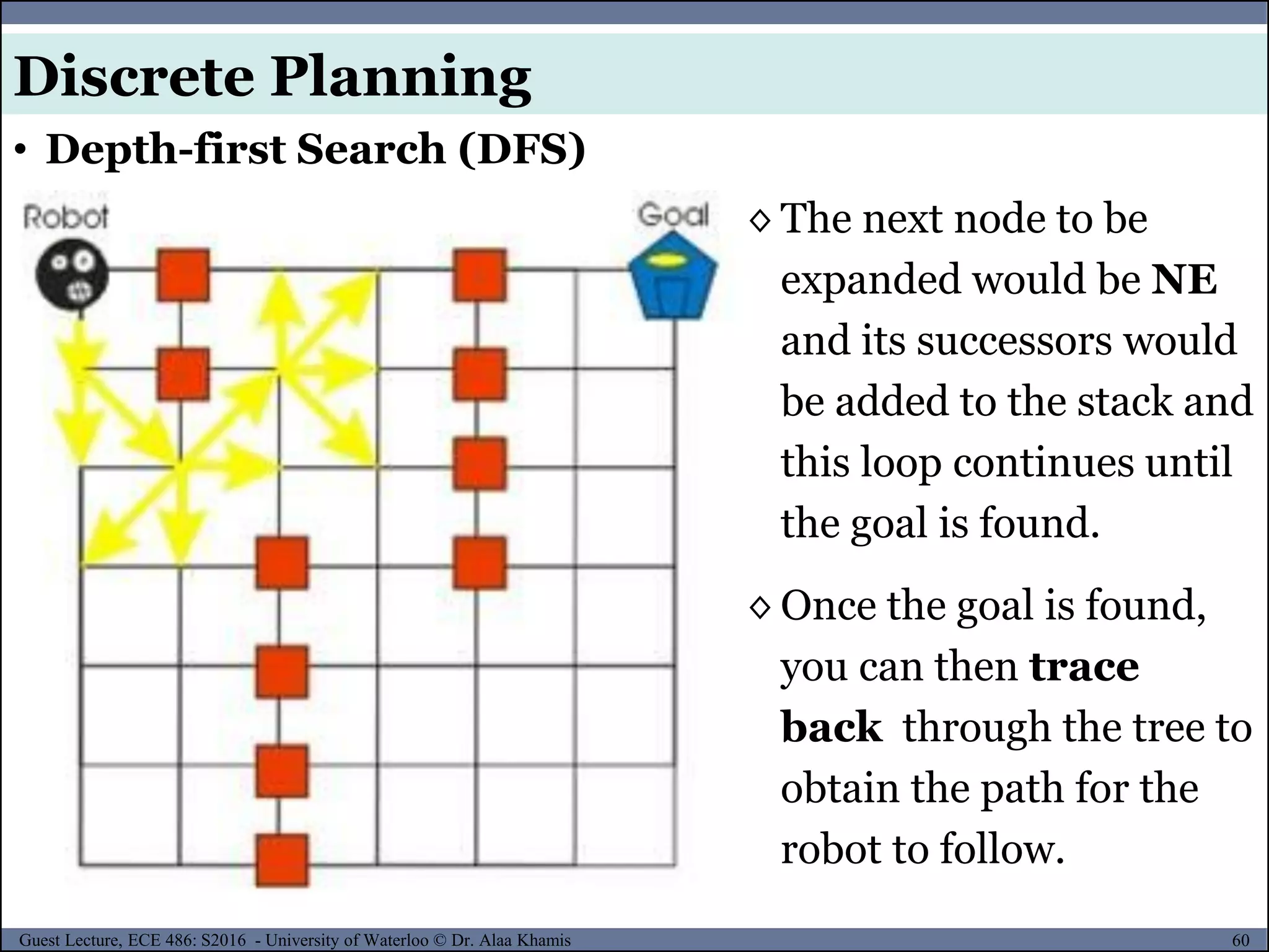
Step 1. Form a queue Q and set it to the initial state (for example, the Root).
Step 2. Until the Q is empty or the goal state is found
do:
Step 2.1 Determine if the first element in the Q is the goal.
Step 2.2 If it is not
Step 2.2.1 remove the first element in Q.
Step 2.2.2 Apply the rule to generate new state(s) (successor states).
Step 2.2.3 If the new state is the goal state quit and return this state
Step 2.2.4 Otherwise add the new state to the end of the queue.
Step 3. If the goal is reached, success; else failure.
[6]
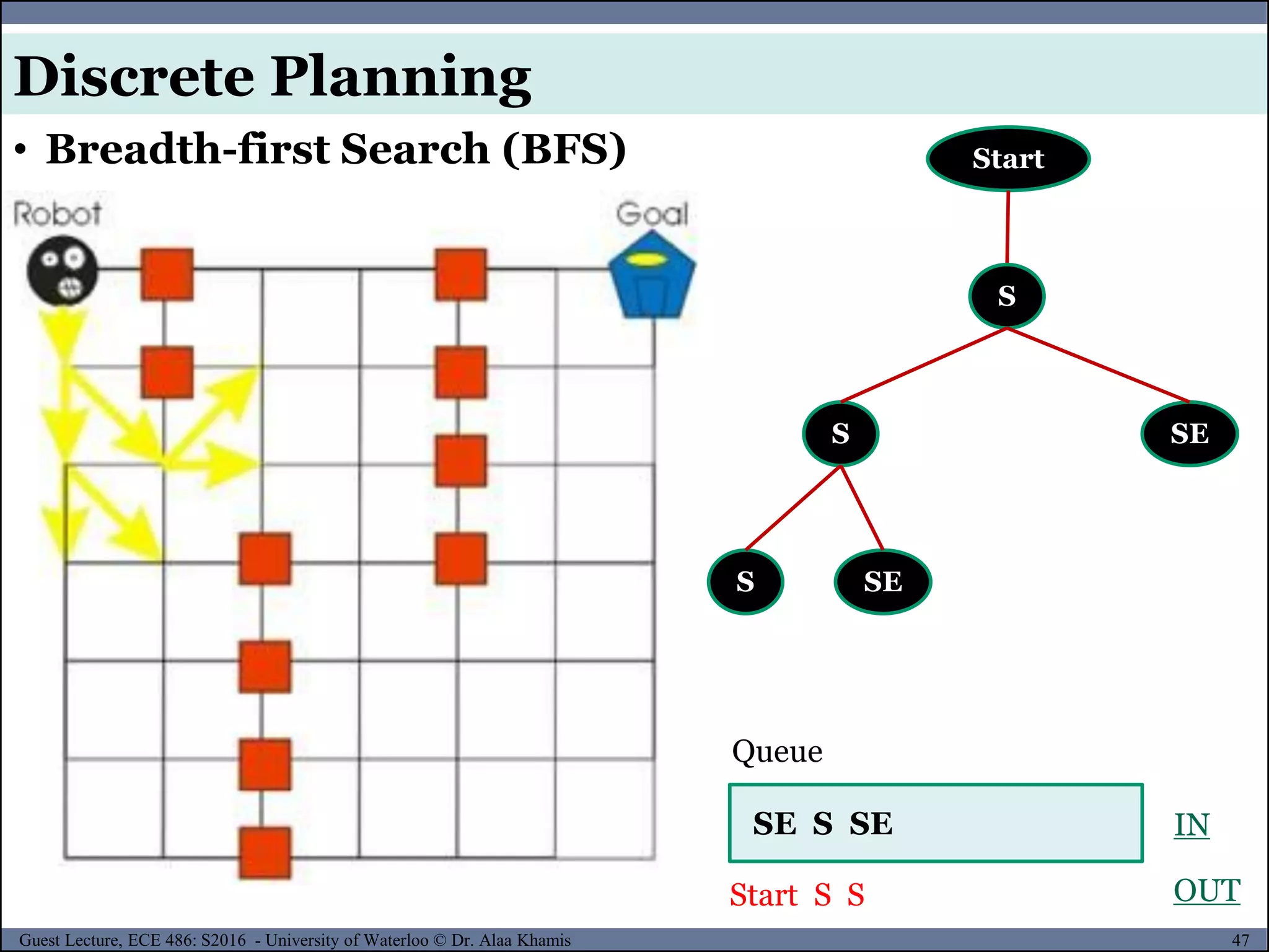
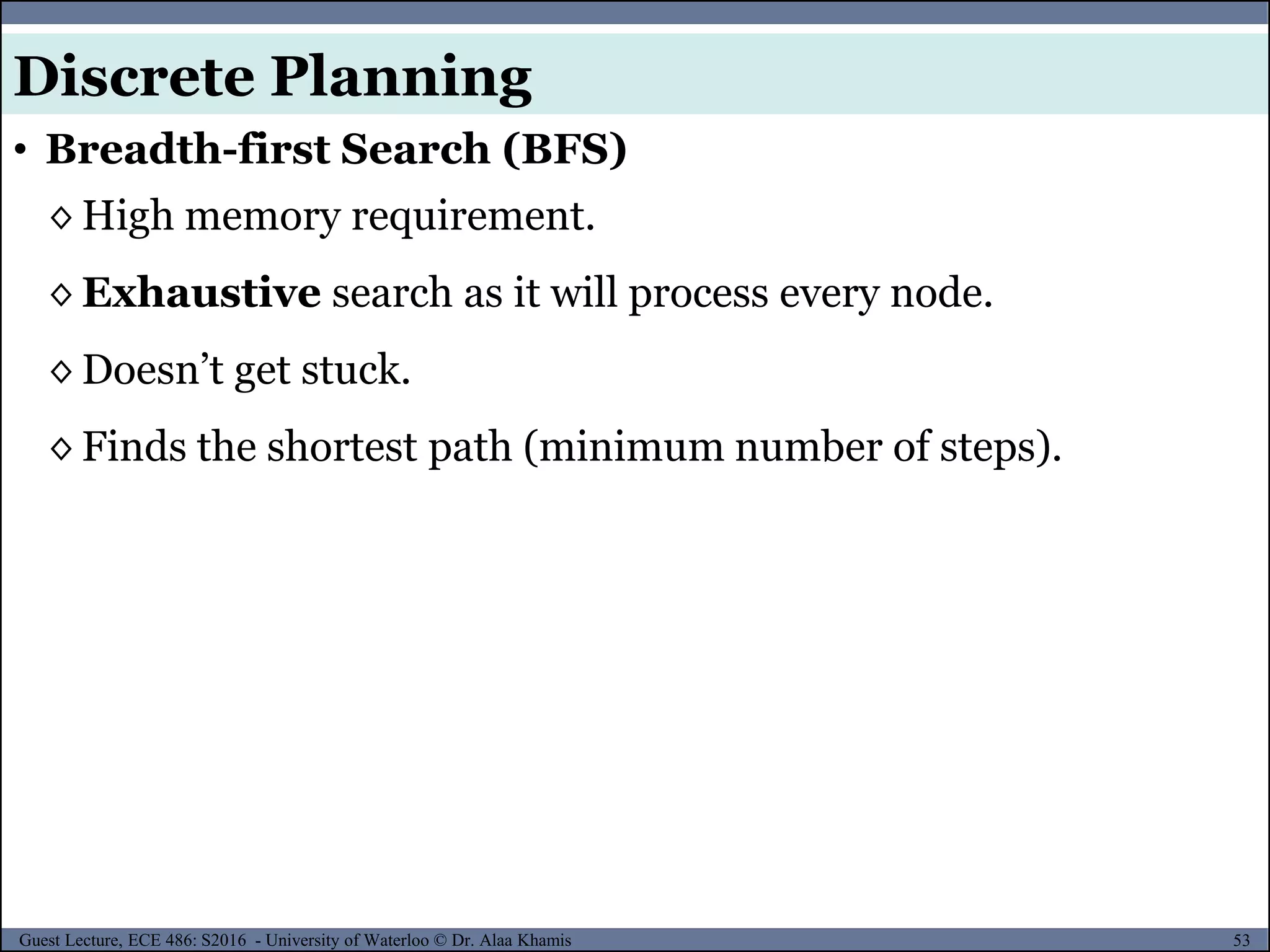
• Breadth-first Search (BFS)
Discrete Planning

◊ BFS uses the queue as data
structure.
◊ Queue is a First-In-First-Out
(FIFO) data structure.
◊ A FIFO means that the node that
has been sitting on the queue for
the longest amount of time is
the next node to be expanded.
Discrete Planning

Start
Queue
Start IN
OUT
Discrete Planning
[7]

Start
S
Queue
S
Start
IN
OUT
Discrete Planning

Start
S
S SE
Queue
SE S
Start S
IN
OUT
Discrete Planning

Start
S
S SE
Queue
SE S SE
Start S S
S SE
IN
OUT
Discrete Planning

Start
S
S SE
Queue
NE E SE S
Start S S SE
S SE E NE
IN
OUT
Discrete Planning

Start
S
S SE
S SE E NE
◊ The FIFO queue continues
until the goal node is found
Discrete Planning

Start
S
S SE
S SE E NE
◊ The path leading to the goal
node (E) is traced back
up the tree which maps
out the directions that the
robot must follow to reach
the goal.
◊ Traveling back up the
tree, we can see that the
robot from the start would
have to go south, then
south east, then east to
reach the goal.
Assume that E is the goal,
Path is: Start SSEE
Discrete Planning

◊ In BFS, every node generated
must remain in memory.
◊ The number of nodes
generated is at most:
O(bd)
where b represents the
maximum branching
factor for each node and d is
the depth one must expand
to reach the goal.
b=2 and d=3
Total # of nodes=23=8
Start
S
S SE
S SE E NE
Discrete Planning

◊ Space complexity: O(bd) (keep every node in memory)
◊ We can see from this that a for very large workspace
where the goal is deep within the workspace, the
number of nodes could expand exponentially and demand
a very large memory requirement.
◊ Time Complexity:
i.e., exponential in d.
2 1
1 .... ( 1)/( 1) ( )d d d
b b b b b O b
       
Discrete Planning

◊ High memory requirement.
◊ Exhaustive search as it will process every node.
◊ Doesn’t get stuck.
◊ Finds the shortest path (minimum number of steps).
Discrete Planning

Step 1. Form a stack S and set it to the initial state (for example, the Root).
Step 2. Until the S is empty or the goal state is found
do:
Step 2.1 Determine if the first element in the S is the goal.
Step 2.2 If it is not
Step 2.2.1 Remove the first element in S.
Step 2.2.2 Apply the rule to generate new state(s) (successor states).
Step 2.2.3 If the new state is the goal state quit and return this state
Step 2.2.4 Otherwise add the new state to the beginning of the stack
Step 3. If the goal is reached, success; else failure.
• Depth-first Search (DFS)
Discrete Planning

Stack (LIFO)
◊ DFS uses the stack as data structure.
◊ Stack is a Last-In-First-Out
(LIFO) data structure.
◊ The stack contains the list of
discovered nodes. The most recent
discovered node is put (pushed) on
top of the LIFO stack.
◊ The next node to be expanded is
then taken (popped) from the top of
the stack and all of its successors are
added to the stack.
http://wiki.ugcnet4cs.in/t/Stack
Discrete Planning

Start
Stack
Start
INOUT
Discrete Planning

Start
S
Stack
SStart
INOUT
Discrete Planning

Stack
SE
S
S
Start
Start
S
S SE
INOUT
Discrete Planning

NE
E
S
SW
S
SE
S
Start
Start
S
S SE
S E NESW
Discrete Planning

◊ The next node to be
expanded would be NE
and its successors would
be added to the stack and
this loop continues until
the goal is found.
◊ Once the goal is found,
you can then trace
back through the tree to
obtain the path for the
robot to follow.
Discrete Planning

◊ Depth first search usually requires a considerably less
amount of memory that BFS.
◊ This is mainly because DFS does not always expand out every
single node at each depth.
◊ However the DFS could continue down an unbounded
branch forever even if the goal is not located on that
branch.
◊ Time Complexity: O(bd)  terrible if d is much larger than
b but if solutions are dense, may be much faster than BFS.
◊ Space Complexity: O(bd), i.e., linear space!
Discrete Planning

◊ Low memory requirement.
◊ Full state space search in that every node is processed, i.e, it’s
exhaustive within its set limits.
◊ Could get stuck exploring infinite paths.
◊ Used if there are many solutions and you need only one.
Discrete Planning

• BFS vs. DFS
BFS DFS
Space Complexity More expensive Less expensive.
Requires only O(d)
space irrespective of
number of children
per node.
Time Complexity More time efficient.
A vertex at lower level
(closer to the root) is
visited first before
visiting a vertex that is
at higher level (far away
from the root)
Less time efficient.
Discrete Planning

DFS is preferred if
◊ The tree is deep;
◊ Solutions occur deeply in the tree;
◊ The branching factor is not excessive.
BFS is preferred if
◊ The branching factor is not too large (hence memory costs);
◊ A solution appears at a relatively shallow level;
◊ No path is excessively deep.
• BFS vs. DFS
Discrete Planning

◊ Blind search finds only one arbitrary solution instead of
the optimal solution.
◊ To find the optimal solution with DFS or BFS, you must not
stop searching when the first solution is discovered. Instead,
the search needs to continue until it reaches all the solutions,
so you can compare them to pick the best.
◊ The strategy for finding the optimal solution is called British
Museum search or brute-force search.
The inventors called this procedure the British Museum
algorithm "... since it seemed to them as sensible as
placing monkeys in front of typewriters in order to
reproduce all the books in the British Museum [5]."
• British Museum Search
Discrete Planning

Dijkstra’s algorithm (Dynamic Programming) is a graph
search algorithm that solves the single-source shortest
path problem for a fully connected graph with nonnegative
edge path costs, producing a shortest path tree.
Dynamic programming (a fancy name for divide-and-
conquer with a table) approaches are based on the recursive
division of a problem into simpler sub-problems.
Dijkstra’s algorithm is uninformed, meaning it does not need to
know the target node before hand and doesn’t use heuristic
information.
• Dijkstra’s Algorithm
Discrete Planning

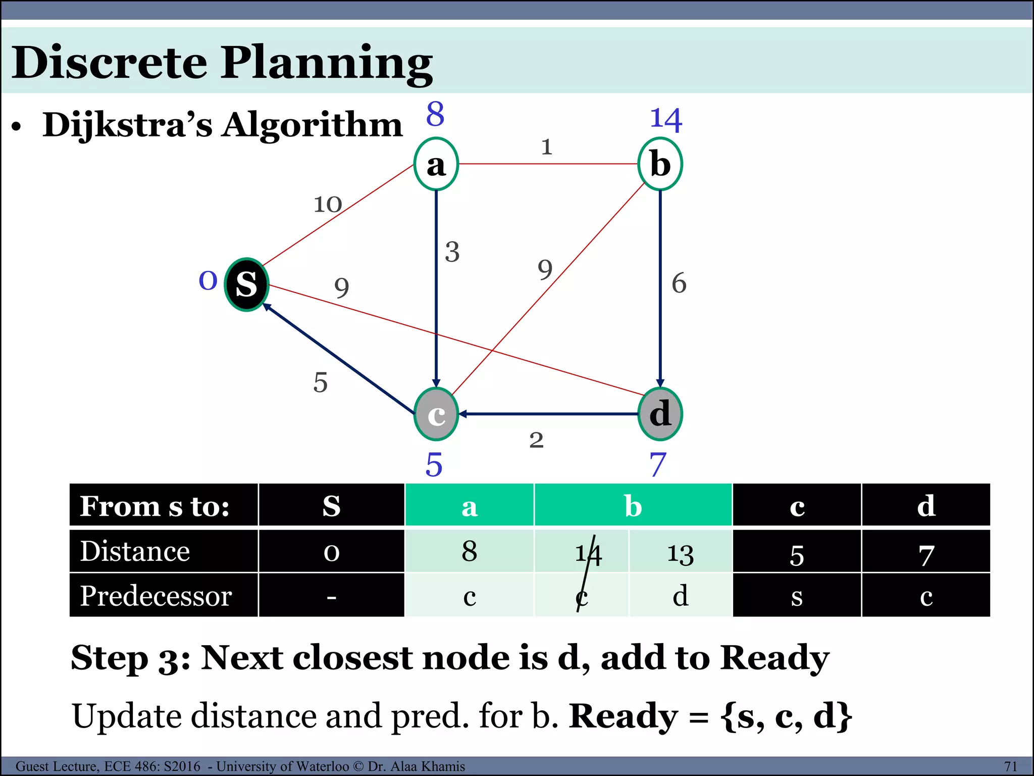
1. Init
Set start distance to 0, dist[s]=0,
others to infinite: dist[i]= (for is),
Set Ready = { } .
2. Loop until all nodes are in Ready
Select node n with shortest known distance that is not in Ready
set Ready = Ready + {n} .
FOR each neighbor node m of n
IF dist[n]+edge(n,m) < dist[m] /* shorter path found */
THEN { dist[m] = dist[n]+edge(n,m); pre[m] = n;}
Discrete Planning

S
c
0
a
d
b

 

10
9
9
3
2
5
6
1
From s to: S a b c d
Distance 0    
Predecessor - - - - -
Step 0: Init list, no predecessors
Ready = {}
[7]
Discrete Planning

S
c
0
a
d
b
10
5 9

10
9
9
3
2
5
6
1
Distance 0 10  5 9
Predecessor - s - s s
Step 1: Closest node is s, add to Ready
Update distances and pred. to all neighbors of s, Ready = {S}
Discrete Planning

S
c
0
a
d
b
8
5 7
14
10
9
9
3
2
5
6
1
Distance 0 10 8 14 5 9 7
Predecessor - s c c s s c
Step 2: Next closest node is c, add to Ready
Update distances and pred. for a and d, Ready = {S, c}
Discrete Planning

S
c
0
a
d
b
8
5 7
14
10
9
9
3
2
5
6
1
Step 3: Next closest node is d, add to Ready
Update distance and pred. for b. Ready = {s, c, d}
Distance 0 8 14 13 5 7
Predecessor - c c d s c
Discrete Planning

S
c
0
a
d
b
8
5 7
14
10
9
9
3
2
5
6
1
Step 4: Next closest node is a, add to Ready
Update distance and pred. for b. Ready = {S, a, c, d}
Distance 0 8 13 9 5 7
Predecessor - c d a s c
Discrete Planning

S
c
0
a
d
b
8
5 7
9
10
9
9
3
2
5
6
1
Step 5: Closest node is b, add to Ready
check all neighbors of s. Ready = {S, a, b, c, d} complete!
Distance 0 8 9 5 7
Predecessor - c a s c
Discrete Planning

Shortest path between s and a is {S, c, a}  length=8
S
c
0
a
d
b
8
5 7
9
10
9
9
3
2
5
6
1
Distance 0 8 9 5 7
◊ dist[a] = 8
◊ pre[a] = c
◊ pre[c] = S
◊ Shortest path:
Sc a,
◊ Length is 8
Discrete Planning

Shortest path between s and b is {S, c, a,b}  length=9
S
c
0
a
d
b
8
5 7
9
10
9
9
3
2
5
6
1 ◊ dist[b] = 9
◊ pre[b] = a
◊ pre[a] = c
◊ pre[c] = S
◊ Shortest path:
Sc a b
Distance 0 8 9 5 7
Discrete Planning

Shortest path between s and d is {S, c}  length=5
S
c
0
a
d
b
8
5 7
9
10
9
9
3
2
5
6
1 ◊ dist[c] = 5
◊ pre[c] = S
◊ Shortest path:
Sc
Distance 0 8 9 5 7
Discrete Planning

Shortest path between s and d is {S, c, d}  length=7
S
c
0
a
d
b
8
5 7
9
10
9
9
3
2
5
6
1 ◊ dist[d] = 7
◊ pre[d] = c
◊ pre[c] = S
◊ Shortest path:
Sc d
Distance 0 8 9 5 7
Discrete Planning

Discrete Planning
As can be seen from previous example, instead of solving
subproblems recursively, solve them sequentially and store their
solutions in a table. The trick is to solve them in the right order
so that whenever the solution to a subproblem is needed, it is
already available in the table [I. Parberry. Problems on algorithms. Prentice-Hall, 1995].

1. Workspace discretized into cells
2. Insert (xinit,yinit) into list OPEN
3. Find all 8-way neighbors to (xinit,yinit) that have not been previously
visited and insert into OPEN
4. Sort neighbors by minimum potential
5. Form paths from neighbors to (xinit,yinit)
6. Delete (xinit,yinit) from OPEN
7. (xinit,yinit) = minPotential(OPEN)
8. GOTO 2 until (xinit,yinit)=goal (SUCCESS) or OPEN empty (FAILURE)
• Best-first
Discrete Planning

+
Goal+
Neighbor
Visited
Obstacle
Local minimum
detected
Best step
• Best-first
Discrete Planning

+
Goal+
Neighbor
Visited
Obstacle
Local minimum
detected

Best step
• Best-first
Discrete Planning

+
Goal+
Neighbor
Visited
Obstacle
Local minimum
detected
Best step
• Best-first
Discrete Planning

◊ It is a kind or mixed depth and breadth first search.
◊ Adds the successors of a node to the expand list.
◊ All nodes on the list are sorted according to the heuristic
values.
◊ Expand most desirable unexpanded node.
◊ Special Case: A*.
• Best-first
Discrete Planning

Pronounced “A-Star”; heuristic algorithm for computing the
shortest path from one given start node to one given goal
node.
The A* search algorithm is a variant of dynamic programming
(Dijkstra) that tries to reduce the total number of states
explored by incorporating a heuristic estimate of the cost to
get the goal from a given state.
• A* Algorithm
Discrete Planning

1. Use a queue to store all the partially expanded paths.
2. Initialize the queue by adding to the queue a zero length path from the root
node to nowhere.
3. Repeat
Examine the first path on the queue.
If it reaches the goal node then success.
Else {continue search}
Remove the first path from the queue.
Expand the last node on this path by one step.
Calculate the cost of these new paths.
Add these new paths to the queue.
• A* Algorithm
Discrete Planning

Sort the queue in ascending order according to the sum of the cost of the
expanded path and the estimated cost of the remaining path for each path.
If more than one path reaches a subnode
Then delete all but the minimum cost path.
Until the goal has been found or the queue is empty.
4. If the goal has been found return success and the path, otherwise return failure.
• A* Algorithm
Discrete Planning

A
S
C E
DB
G4
3
3
5
3
5
3
2
4
F
10.5
8.5 5.7 2.8
0
3710.3
S
A B
C
E
D
B
G
11.5
11.7
11.8
12
12.3
17.3
21
• A* Algorithm
Discrete Planning

Source:
http://en.wikipedia.org/wiki/File:Astar_progress_animation.gif
• A* Algorithm
Discrete Planning

◊ This algorithm may look complex since there seems to be the
need to store incomplete paths and their lengths at various
places.
◊ However, using a recursive best-first search
implementation can solve this problem in an elegant way
without the need for explicit path storing.
◊ The quality of the lower bound goal distance from each node
greatly influences the timing complexity of the algorithm.
◊ The closer the given lower bound is to the true
distance, the shorter the execution time.
• A* Algorithm
Discrete Planning

Outline

The road map approach consists of generating connecting
cells within mobile robot’s free space into a network of one-
dimensional curves called a road map.
 Properties of a Roadmap:
◊ Accessibility: there exists a collision-
free path from the start to the road map
◊ Departability: there exists a collision-
free path from the roadmap to the goal.
◊ Connectivity: there exists a collision-
free path from the start to the goal (on
the roadmap). A roadmap exists  A
path exists
• Road map
Combinatorial Planning

Road Map Approaches
Voronoi Diagrams
Visibility Graph
Maklink
Free Way Net
Silhouette
…
• Road map

◊ Suppose someone gives you a CSPACE with polygonal
obstacles.
◊ Visibility graph is formed by connecting all “visible”
vertices, the start point and the end point, to each other.
◊ For two points to be “visible” no obstacle can exist between
them, i.e., paths exist on the perimeter of obstacles.
• Road map: Visibility Graph

1. Start with a map of the world, draw lines of sight from the
start and goal to every “corner” of the world and
vertex of the obstacles, not cutting through any
obstacles.
2. Draw lines of sight from every vertex of every obstacle
like above. Lines along edges of obstacles are lines of sight
too, since they don’t pass through the obstacles.
3. If the map was in Configuration space, each line potentially
represents part of a path from the start to the goal.

◊ First, draw lines of sight from the start and goal to all “visible”
vertices and corners of the world.
S
G

◊ Second, draw lines of sight from every vertex of every obstacle
like before. Remember lines along edges are also lines of
sight.
G
S

sight.
G
S

◊ Repeat until you’re done.
◊ Search the graph of these lines for the shortest path (using
Dijkstra algorithm for example).
S
G

• Cell Decomposition
The idea behind cell decomposition is
to discriminate between geometric
areas, or cells, that are free and areas
that are occupied by objects.
Cell Decomposition
Exact Cell
Decomposition
Approximate Cell
Decomposition
Adaptive
Decomposition
Fixed
Decomposition

◊ Divide environment into simple, connected regions called
“cells”.
Any path
within one cell
is guaranteed
to not intersect
any obstacle
• Exact Cell Decomposition

◊ Determine which
opens cells are
adjacent.

◊ Find the cells in
which the initial
and goal
configurations lie
and search for a
path in the
connectivity graph
to join the initial
and goal cell.

◊ Construct the connectivity
graph.
The connectivity graph of cells defines
a roadmap

◊ From the sequence of cells
found with an appropriate
searching algorithm,
compute a path within each
cell, for example, passing
through the midpoints of
the cell boundaries or by
a sequence of wall-
following motions and
movements along straight
lines. The connectivity graph of cells defines
a roadmap

◊ From the sequence of cells
found with an appropriate
searching algorithm,
compute a path within each
cell, for example, passing
through the midpoints of
the cell boundaries or by
a sequence of wall-
following motions and
movements along straight
lines. The graph can be used to find a path
between any two configurations

◊ The key disadvantage of exact cell decomposition is that the
number of cells and, therefore, overall path planning
computational efficiency depends upon the density and
complexity of objects in the environment, just as with
road map-based systems.
◊ Practically speaking, due to complexities in implementation,
the exact cell decomposition technique is used relatively
rarely in mobile robot applications, although it remains a
solid choice when a lossless representation is highly desirable,
for instance to preserve completeness fully.

• Approximate Cell Decomposition
◊ By contrast, approximate cell decomposition is one of the
most popular techniques for mobile robot path planning.
◊ This is partly due to the popularity of grid-based
environmental representations.
Approximate Cell
Decomposition
Adaptive
Decomposition
Fixed
Decomposition

• Fixed Decomposition
1. Define a discrete grid in C-Space
2. Mark any cell of the grid that intersects obstacles as blocked
3. Find path through remaining cells by using (for example) A*
(e.g., use Euclidean distance as heuristic)
◊ Cannot be complete as described so far. Why?
S
G

S
G
• Fixed Decomposition
The key disadvantage of this
approach stems from its inexact
nature. It is possible for narrow
passageways to be lost during
such a transformation.
Cannot find a path in this case even
though one exists.

• Adaptive Decomposition
1. Distinguish between Cells that are entirely contained in
obstacles (FULL) and Cells that partially intersect obstacles
(MIXED)
2. Try to find a path using the current set of cells.
3. If no path found:
Subdivide the MIXED cells and try again with the new set
of cells.

S
G

• Approximate Cell Decomposition
◊ Pros:
 Limited assumptions on obstacle configuration
 Approach used in practice
 Find obvious solutions quickly
◊ Cons:
 No clear notion of optimality (“best” path)
 Trade-off completeness/computation
 Still difficult to use in high dimensions

Outline

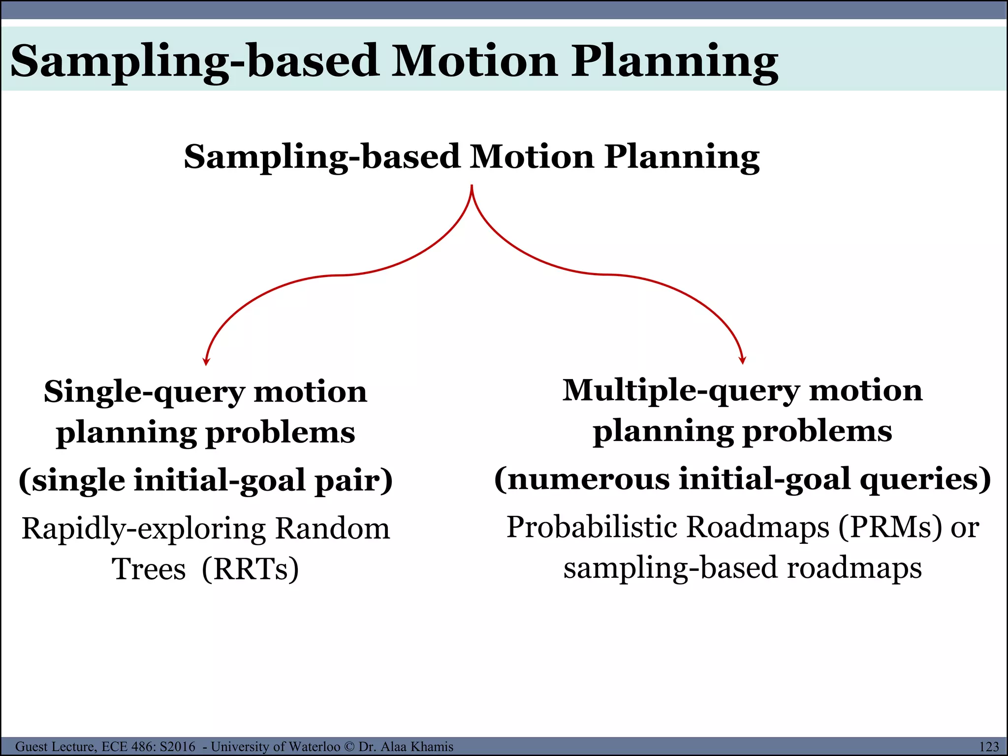
• The main idea of sampling-based motion planning is to avoid
the explicit construction of 𝒞obs, and instead conduct a search
that probes the C-space with a sampling scheme.
Sampling-based Motion Planning
Geometric
Models
Collision
Detection
Sampling-based Motion
Planning Algorithm
Discrete
Searching
C-Space
Sampling
[2]
• The sampling-based planning philosophy uses collision
detection as a “black box” that separates the motion planning
from the particular geometric and kinematic models.
• C-space sampling and discrete planning (i.e., searching) are
performed.

Multiple-query motion
planning problems
(numerous initial-goal queries)
Probabilistic Roadmaps (PRMs) or
sampling-based roadmaps
Single-query motion
planning problems
(single initial-goal pair)
Rapidly-exploring Random
Trees (RRTs)

• Probabilistic Roadmaps (PRMs)
Given: G(V,E) represents a
topological graph in which V is a
set of vertices and E is the set of
paths that map into 𝒞free.
Under the multiple-query philosophy, motion planning is
divided into two phases of computation:
Preprocessing/Learning Phase Query Phase
Build G in a way that is useful for
quickly answering future queries. For
this reason, it is called a roadmap,
which in some sense should be
accessible from every part of 𝒞free.
roadmap
query
(qinit,qgoal) pair
Path
[2]

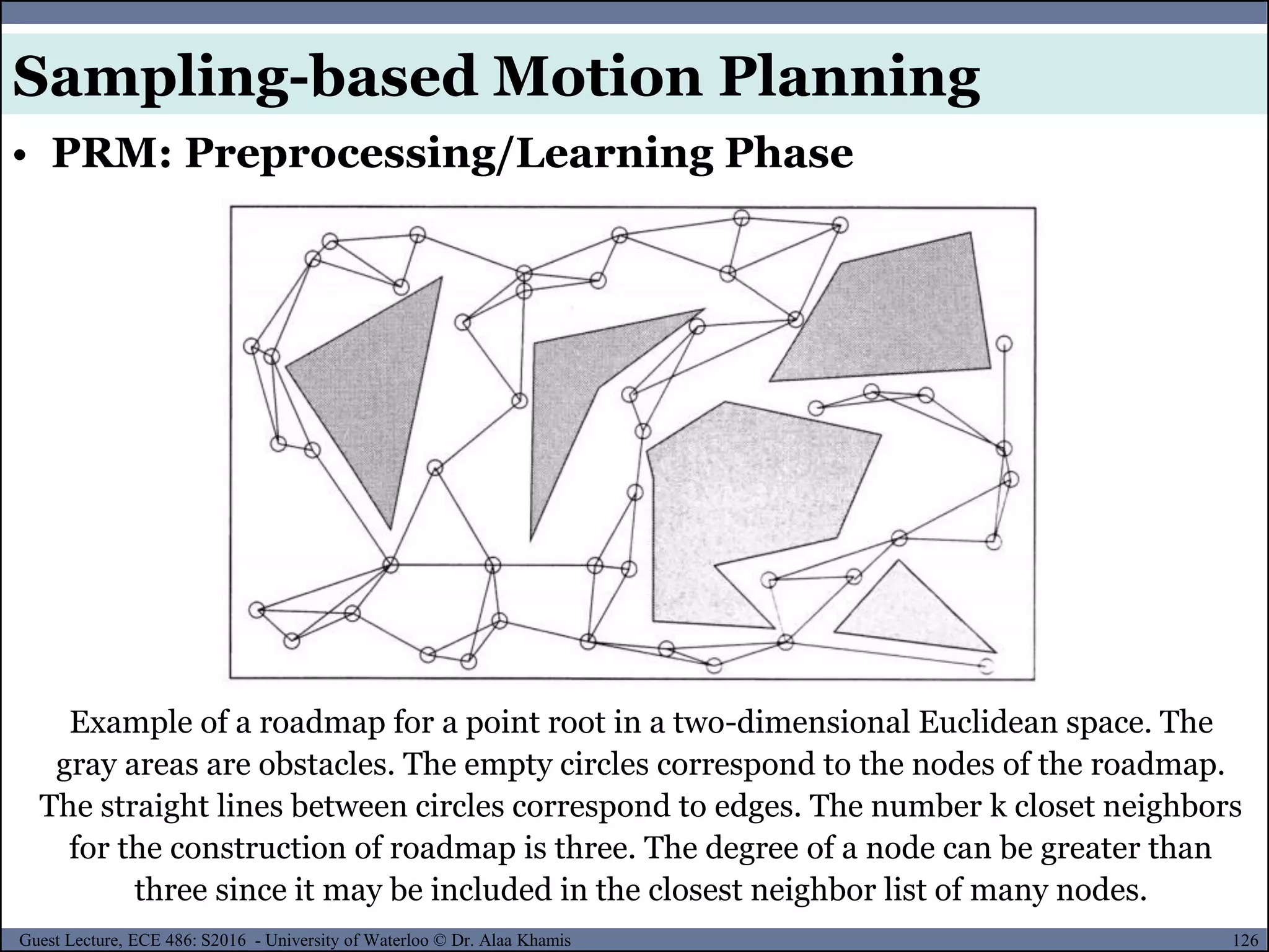
• PRM: Preprocessing/Learning Phase
The sampling-based roadmap
is constructed incrementally by
attempting to connect each
new sample, (i), to nearby
vertices in the roadmap
Note that i is not incremented if (i) is in collision. This forces i
to correctly count the number of vertices in the roadmap.
[2]
Possible selection methods:
 Nearest K;
 Radius;
 Visibility
 …

• PRM: Preprocessing/Learning Phase
Example of a roadmap for a point root in a two-dimensional Euclidean space. The
gray areas are obstacles. The empty circles correspond to the nodes of the roadmap.
The straight lines between circles correspond to edges. The number k closet neighbors
for the construction of roadmap is three. The degree of a node can be greater than
three since it may be included in the closest neighbor list of many nodes.

• PRM: Query Phase
◊ Given an initial position and a final
position or (qinit,qgoal) pair, the roadmap
should compute a collision-free path
between these two configurations.
◊ First, we create new nodes for each of the initial and final
position we add them to the graph after a collision test if
needed.
◊ Then, we try to connect the two nodes to the graph to any of
their neighbors, just like as we did in the learning phase.
◊ If the path planner fails to compute a feasible path between
the new nodes and the existing nodes, the query phase fails.

• PRM: Summary
a) A set of random sample is
generated in the configuration
space. Only collision-free samples
are retrained.
b) Each sample is connected to its
nearest neighbors using a simple,
straight-line path. If such a path
causes a collision, the
corresponding samples are not
connected in the roadmap
[4]

• PRM: Summary
c) Since the initial roadmap contains
multiple connected components,
additional samples are generated and
connected to the roadmap.
d) A path from qinit to qgoal is found by
connected qinit and qgoal to the
roadmap and then searching this
augmented roadmap for a path from
qinit to qgoal
[4]

• PRM: Summary
For reading: http://spectrum.ieee.org/automaton/robotics/robotics-software/custom-processor-speeds-up-robot-motion-
planning-by-factor-of-1000/?utm_source=RoboticsNews&utm_medium=Newsletter&utm_campaign=RN07052016

Outline

The potential field method incrementally explores 𝓒free,
searching for a path from qinit to qfinal. At termination, this planner
returns a single path.
Potential field path planning creates a field, or gradient, across
the robot’s map that directs the robot to the goal position from
multiple prior positions.
Robot
Goal
Obstacle
The potential field method
treats the robot as a point
under the influence of an
artificial potential
field, U(q).
Potential Field Method

The robot moves by following the field, just as a ball would roll
downhill. The goal (a minimum in this space) acts as an
attractive force on the robot and the obstacles act as peaks, or
repulsive forces. The superposition of all forces is applied to the
robot.
Start
+
Goal
Obstacle

The artificial potential field smoothly guides the robot
toward the goal while simultaneously avoiding known
obstacles.
Attraction
Repulsion

Assume that the robot is a point, thus the robot’s orientation is
neglected and the resulting potential field is only 2D (x,y).
Assume a differentiable potential field function U(q).
The related artificial force acting at the position q=(x,y) is
Robot
Goal
Obstacle
q=(x,y)
)()( qUqF 
where denotes the
gradient vector of U at position q.
)(qU

















y
U
x
U
qU )(

The potential field acting on the robot is then computed as the
sum of the attractive field of the goal and the repulsive
fields of the obstacles:
)()()( qUqUqU repatt 
◊ Uatt is the “attractive” potential --- move to the goal
◊ Urep is the “repulsive” potential --- avoid obstacles

◊ katt is a positive scaling factor
◊ dgoal denotes the Euclidean distance
Quadratic Potential
)(.
2
1
)( 2
qdkqU goalattatt 
goalqq 
where
• Attractive Potential

).(.)()( goalattgoalgoalattattatt qqkddkqUqF 
This converges linearly
toward 0 as the robot
reaches the goal
This attractive potential is differentiable, leading to the
attractive force:
)(.
2
1
)( 2
qdkqU goalattatt 
NOTE: q is a vector
corresponding to a
position in the
workspace







y
x
q
q
q
• Attractive Potential

◊ The idea behind the repulsive potential is to generate a force
away from all known obstacles.
◊ This repulsive potential should
be very strong when the robot
is close to the object, but
should not influence its
movement when the robot is far
from the object.
• Repulsive Potential


















*
*
2
*
)(0
)(
1
)(
1
.
2
1
)(
Qqd
Qqd
Qqd
k
qU
obj
obj
obj
rep
rep
◊ krep is again a scaling factor,
◊ dobj is the minimal distance from q to the object and
◊ Q* is the distance of influence of the object.
where


















*
*
2
*
)(0
)(
1
)(
1
.
2
1
)(
Qqd
Qqd
Qqd
k
qU
obj
obj
obj
rep
rep
◊ The repulsive potential
function is positive or
zero and tends to
infinity as gets closer to
the object.


















*
*
2
*
)(0
)(
1
)(
1
.
2
1
)(
Qqd
Qqd
Qqd
k
qU
obj
obj
obj
rep
rep
The repulsive force is

















*
*
2*
)(0
)(.
1
.
1
)(
1
.
)()(
Qqd
Qqdd
dQqd
k
qUqF
obj
objobj
objobj
rep
reprep
where denotes the partial derivate vector of the distance
from the point subject to potential (PSP or q) to he obstacle or
object.
objd
T
objobj
obj
y
d
x
d
d












 ,

)()()()( qUqFqFqF repatt 
+ =
A first-order optimization
algorithm such as gradient
descent (also known as
steepest descent) can be
used to minimize this function
by taking steps proportional
to the negative of the gradient.
• The resulting force

◊ Gradient descent is a first-order optimization algorithm.
◊ To find a local minimum of a function using gradient descent,
one takes steps proportional to the negative of the
gradient (or of the approximate gradient) of the function at
the current point.
GradientDescent(xinit, xfinal, -f)
while xinitxfinal
xn+1 = xn -nf(xn), n0
end
• Gradient Descent or Steepest Descent

where
GradientDescent(xo, xfinal, -f)
while xoxfinal
xn+1 = xn -nf(xn), n0
end
 >0 is a small enough number.
Note that the step size  must be small enough to ensure that
we do not collide with an obstacle or overshoot our goal position.
The value of the step size γ is allowed to change at every
iteration.

We have:
F(xo)  F(x1)  F(x2) … F(xfinal)
GradientDescent(xo, xfinal, -f)
while xoxfinal
xn+1 = xn -nf(xn), n0
end
so hopefully the sequence converges to the desired local
minimum xfinal. Note that in practice, we will stop within some
tolerance (like  ) of the final position to account for positional
uncertainties, etc.

A Parabolic Well for Attracting to Goal
Parabolic Well Goal & Exponential Source for Obstacle
• Exemples

Parabolic Well Goal & Two Exponential Source Obstacles
Parabolic Well Goal & Two Exponential Source Obstacles
Motion Planning Solvers
• Exemples

Parabolic Well Goal & Multiple Exponential Source Obstacles
Modeling Walls in a Closed Workspace
• Exemples

◊ Trap situations due to local minima: One major
problem with this algorithm is preventing local minima.
These are the points where the attractive and repulsive forces
cancel each others. Local minima can exist by a variety of
different obstacle configurations. There are several techniques
to decrease or even avoid the local minima.
• Problems of Potential Field Method

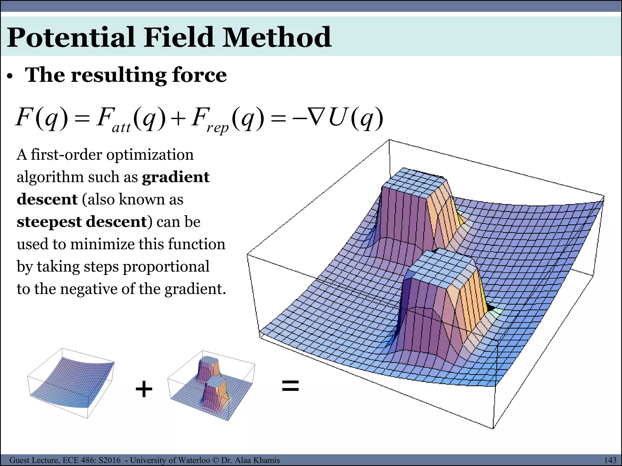
The configuration qmin is a local minimum in the potential field.
At qmin the attractive force exactly cancels the repulsive fore and
the planner fails to make further progress.
[4]

Local Minimum Problem with the Charge Analogy
◊ The robot can get
stuck in local
minima.
◊ In this case the
robot has reached
a spot with zero
force (or a level
potential), where
repelling and
attracting forces
cancel each
other out.
◊ So the robot will
stop and never
reach the goal.

◊ No passage between closely spaced obstacles: There is
no passage between closely spaced obstacles; as the
repulsive forces due to the first and the second
obstacle add up to a force pointing away from the
passage. Thus the robot will either approach the passage
further or it will turn away.

◊ Oscillations in Narrow Passages: The robot experience
repulsive forces simultaneously from opposite sides
when traveling in narrow corridors resulting in an unstable
motion.
◊ The scenario where the goal is located near an obstacle
such that the repulsive force can be larger than the attractive
force resulting in a motion away from the goal instead of
reaching it.

Outline

◊ A path is defined as the
collection of a sequence of
configurations a robot
makes to go from one place to
another without regard to the
timing of these
configurations.
Sequential robot movements in a path
◊ A trajectory is related to the timing at which each part of the
path must be attained.
◊ As a result, regardless of when points B and C in the figure are
reached, the path is the same, whereas depending on how fast
each portion of the path is traversed, the trajectory may differ.
Same Path Different
Trajectories
Trajectory Planning
• Path versus Trajectory
[8]

◊ The points at which the robot may be on a path and on a
trajectory at a given time may be different, even if the robot
traverses the same points.
◊ On a trajectory, depending on the velocities and
accelerations, points B and C may be reached at different
times, creating different trajectories.
◊ In this lecture, we are not only concerned about the path a
robot takes, but also its velocities and accelerations.
Trajectory Planning
• Basics: Path versus Trajectory
[8]

• Basics: Joint-space Motion Description




















1000
zpzazozn
ypyayoyn
xpxaxoxn




















6
5
4
3
2
1
θ
θ
θ
θ
θ
θ
Inverse Kinematics
Joint ValuesDesired End-effector Pose B
Joint Controllers
New Pose
B
◊ In this case, although the robot will eventually reach the
desired position, but as we will see later, the motion between
the two points is unpredictable.
◊ The joint values calculated using
inverse kinematics are used by the
controller to drive the robot joints to
their new values and, consequently,
move the robot arm to its new position.
Trajectory Planning
[8]

Sequential motions of a robot to follow a straight line
• Basics: Cartesian-space Motion Description
◊ Now assume that a straight line is drawn between points A
and B, and it is desirable to have the robot move from point A
to point B in a straight line.
◊ To do this, it will be necessary to divide the line into small
segments, as shown above and to move the robot through all
intermediate points.
Trajectory Planning
[8]

◊ To accomplish this task, at each intermediate location, the
robot’s inverse kinematic equations are solved, a set of joint
variables is calculated, and the controller is directed to drive
the robot to those values. When all segments are completed,
the robot will be at point B, as desired.
◊ However, in this case, unlike the
joint-space case, the motion is
known at all times.
◊ The sequence of movements the
robot makes is described in
Cartesian-space and is converted
to joint-space at each segment.
Sequential motions of a robot to follow
a straight line
Trajectory Planning
[8]

◊ Cartesian-space trajectories are very easy to visualize. Since
the trajectories are in the common Cartesian space in which we
all operate, it is easy to visualize what the end-effector’s
trajectory must be.
◊ However, Cartesian-space
trajectories are
computationally
expensive and require a
faster processing time
for similar resolution than
joint-space trajectories.
Sequential motions of a robot to follow
a straight line
Trajectory Planning
[8]

◊ Although it is easy to visualize the trajectory, it is difficult to
visually ensure that singularities will not occur.
For example, consider the situation shown here.
◊ If not careful, we may specify a trajectory that requires the
robot to run into itself or to reach a point outside of the
work envelope—which, of course, is impossible-and yields
an unsatisfactory solution.
The trajectory specified
in Cartesian coordinates
may force the robot to
run into itself.
The trajectory may
require a sudden change
in the joint angles.
Trajectory Planning
[8]

• Basics:
Given: a simple 2-DOF robot (mechanism)
Required:
2-DOF Mechanism
Move the robot from point A to point B.
Suppose that:
At initial point A: =200 & =300.
At final point B: =400 & =800.
Both joints of the robot can move at the maximum rate of 10
degrees/sec.
Trajectory Planning
[8]

• Joint-space, Non-normalized Movements:
One way to move the robot from point A to B is to run both
joints at their maximum angular velocities. This means
that at the end of the second time interval, the lower link of the
robot will have finished its motion, while the upper link
continues for another three seconds, as shown here:
Joint-space, non-normalized movements of a 2-DOF Mechanism
The path is irregular, and
the distances traveled by the
robot’s end are not uniform.
Trajectory Planning
[8]

• Basics: Joint-space, Normalized Movements
The motions of both joints of the robot are normalized such that
the joint with smaller motion will move proportionally slower so
that both joints will start and stop their motion simultaneously.
In this case, both joints move at different speeds, but move
continuously together.  changes 4 degrees/second while 
changes 10 degrees/second.
Joint-space, normalized movements of a 2-DOF Mechanism
The segments of the
movement are much more
similar to each other than
before, but the path is still
irregular (and different
from the previous case)
Trajectory Planning
[8]

• Basics: Cartesian-space Movements
Now suppose we want the robot’s hand to follow a known path
between points A and B, say, in a straight line.
The simplest solution would be to draw a line between points A
and B, divide the line into, say, 5 segments, and solve for
necessary angles  and  at each point. This is called
interpolation between points A and B.
Cartesian-space movements of a 2-DOF Mechanism
The path is a straight line,
but the joint angles are not
uniformly changing.
Trajectory Planning
[8]

◊ Although the resulting motion is a straight (and consequently,
known) trajectory, it is necessary to solve for the joint
values at each point.
◊ Obviously, many more points must be calculated for better
accuracy; with so few segments the robot will not exactly
follow the lines at each segment.
◊ This trajectory is in Cartesian-
space since all segments of the
motion must be calculated based
on the information expressed in a
Cartesian frame.
Cartesian-space movements
Trajectory Planning
[8]

◊ In this case, it is assumed that the robot’s actuators are
strong enough to provide the large forces necessary to
accelerate and decelerate the joints as needed. For
example, notice that we are assuming the arm will be
instantaneously accelerated to have the desired velocity right
at the beginning of the motion in segment 1.
◊ If this is not true, the
robot will follow a
trajectory different
from our assumption; it
will be slightly behind as
it accelerates to the
desired speed.
Trajectory Planning
[8]

◊ Note how the difference between two consecutive values is
larger than the maximum specified joint velocity of 10
degrees/second (e.g., between times 0 and 1, the joint must
move 25 degrees).
◊ Obviously, this is not attainable. Also note how, in this case,
joint 1 moves downward first before moving up.
Cartesian-space movements of a 2-DOF Mechanism
!!
Trajectory Planning
[8]

◊ Trajectory planning with an acceleration/deceleration
regiment:
Divide the segments differently by starting the arm with
smaller segments and, as we speed up the arm, going at a
constant cruising rate and finally decelerating with
smaller segments as we approach point B.
Accelerate
Constant cruising rate
Decelerate
For each time interval t:
Acceleration: a
Segment: x=(1/2).at2
Cruising velocity of v=at
Trajectory Planning

◊ Trajectory planning with an acceleration/deceleration
regiment:
Of course, we still need to solve the inverse kinematic
equations of the robot at each point, which is similar to the
previous case.
However, in this case, instead of dividing the straight line AB
into equal segments, we may divide it based on x=(1/2).at2
until such time t when we attain the cruising velocity of v=at.
Similarly, the end portion of the motion can be divided based
on a decelerating regiment.
Trajectory Planning
[8]

◊ Another variation to this trajectory planning is to plan a path
that is not straight, but one that follows some desired path,
for example a quadratic equation.
To do this, the coordinates of each segment are calculated based
on the desired path and are used to calculate joint variables at
each segment; therefore, the trajectory of the robot can be
planned for any desired path.
A case where straight line
path is not recommended.
Trajectory Planning
[8]

Outline

◊ In this application, the initial location and orientation of the
robot are known and, using the inverse kinematic equations,
the final joint angles for the desired position and orientation
are found.
◊ However, the motions of each joint of the robot must be
planned individually.
• 3rd Order Polynomial
Inverse Kinematics
―Initial Location and
orientation of the robot
―Initial Joint Angles
―Desired Location and
orientation of the robot.
Final Joint Angles
Joint-Space Trajectory Planning

◊ Consider one of the joints,
At the beginning of the motion segment at time ti
The joint angle is i
following 3rd order polynomial trajectoryi f
3
3
2
21)( tctctcct o 
4 Unknowns: 321 &,, cccco
4 pieces of information:
0)(
0)(
)(
)(




f
i
ff
ii
t
t
t
t







◊ Consider one of the joints,
following 3rd order polynomial trajectoryi f
3
3
2
21)( tctctcct o 
Taking the first derivative of the polynomial:
Substituting the initial and final conditions:
2
321 32)( tctcct 
In matrix form









































3
2
1
2
32
3210
0010
1
0001
c
c
c
c
tt
ttt
θ
θ
θ
θ o
ff
fff
f
i
f
i

032)(
0)(
)(
)(
2
321
1
3
3
2
21




fff
i
ffffof
ioi
tctcct
ct
tctctcct
ct







◊ By solving these four equations simultaneously, we get the
necessary values for the constants. This allows us to calculate
the joint position at any interval of time, which can be
used by the controller to drive the joint to position. The same
process must be used for each joint individually, but they are
all driven together from start to finish.
◊ Applying this third-order polynomial to each joint motion
creates a motion profile that can be used to drive each joint.









































3
2
1
2
32
3210
0010
1
0001
c
c
c
c
tt
ttt
θ
θ
θ
θ o
ff
fff
f
i
f
i


[8]

◊ If more than two points are specified, such that the robot will
go through the points successively, the final velocities and
positions at the conclusion of each segment can be used
as the initial values for the next segments.
◊ Similar third-order polynomials can be used to plan each
section. However, although positions and velocities are
continuous, accelerations are not, which may cause problems.

◊ Example: It is desired to have the first joint of a 6-axis robot
go from initial angle of 30o to a final angle of 75o in 5 seconds.
Using a third-order polynomial, calculate the joint angle at 1, 2,
3, and 4 seconds.
◊ Given:
0)(
0)(
75)(
30)(




f
i
f
i
t
t
t
t






5
0


f
i
t
t
◊ Required:
4and1,2,3at t
[8]

◊ Example (cont’d):
◊ Solution: Substituting the boundary conditions:











0)5(3)5(2)(
0)(
75)5()5()5()(
30)(
2
321
1
3
3
2
21
ccct
ct
cccct
ct
f
i
of
oi

















032)(
0)(
)(
)(
2
321
1
3
3
2
21
fff
i
ffffof
ioi
tctcct
ct
tctctcct
ct





 
72.0,4.5,0,30 321  cccco

[8]

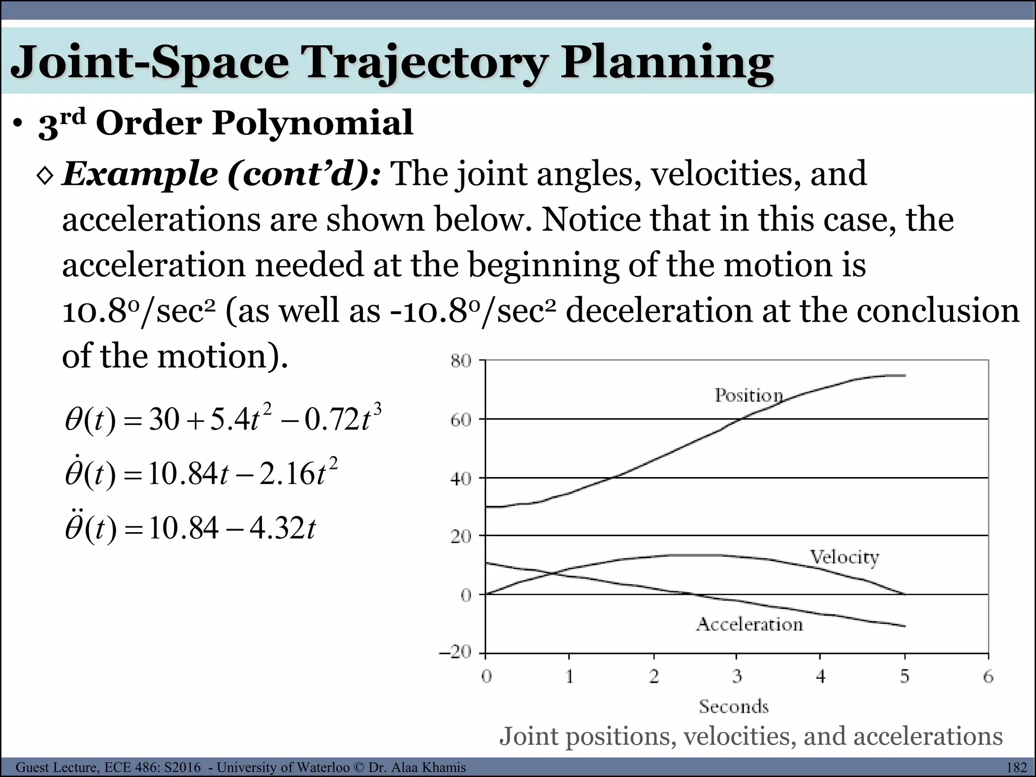
◊ Example (cont’d): This results in the following cubic
polynomial equation for position as well as the velocity and
acceleration equations for joint 1:
tt
ttt
ttt
32.484.10)(
16.284.10)(
72.04.530)(
2
32








Substituting the desired time intervals into the motion
equation will result in:
oooo
32.70)4(,16.59)3(,84.45)2(,68.34)1(  
[8]

◊ Example (cont’d): The joint angles, velocities, and
accelerations are shown below. Notice that in this case, the
acceleration needed at the beginning of the motion is
10.8o/sec2 (as well as -10.8o/sec2 deceleration at the conclusion
of the motion).
tt
ttt
ttt
32.484.10)(
16.284.10)(
72.04.530)(
2
32








Joint positions, velocities, and accelerations

◊ Specifying the initial and ending positions, velocities, and
accelerations of a segment yields six pieces of information,
enabling us to use a fifth-order polynomial to plan a
trajectory, as follows:
3
5
2
432
4
5
3
4
2
321
5
5
4
4
3
3
2
21
201262)(
5432)(
)(
tctctcct
tctctctcct
tctctctctcct o








These equations allow us to calculate the coefficients of a fifth-
order polynomial with position, velocity, and acceleration
boundary conditions.
• 5th Order Polynomial
[8]

◊ Example: Repeat Example-1, but assume the initial
acceleration and final deceleration will be 5o/sec2.
2
2
/sec5/sec075
/sec5/sec030
o
f
o
f
o
f
o
i
o
i
o
i






Substituting in the following equations will result in:
◊ Solution: From Example-1 and the given accelerations, we
have:








3
5
2
432
4
5
3
4
2
321
5
5
4
4
3
3
2
21
201262)(
5432)(
)(
tctctcct
tctctctcct
tctctctctcct o




 
0464.058.06.1
5.2030
543
21


ccc
ccco
[8]

◊ Example (cont’d): This results in the following motion
equations:
32
432
5432
928.09.66.95)(
232.032.28.45)(
0464.058.06.15.230)(
tttt
ttttt
ttttt








Joint positions, velocities, and accelerations
[8]

◊ To ensure that the robot’s accelerations will not exceed its
capabilities, acceleration limits may be used to calculate the
necessary time to reach the target.
Joint positions, velocities, and
accelerations
In example-2:
The maximum acceleration is
8.7o/sec2< max

0and0For  fi  
 
 2max
6
if
if
tt 




 
 
8.10
05
30756
2max




sec/7.8max
o

[8]

Outline

• Cartesian-space trajectories relate to the motions of a robot
relative to the Cartesian reference frame, as followed by the
position and orientation of the robot’s hand.
• In addition to simple straight-line trajectories, many other
schemes may be deployed to drive the robot in its path between
different points.
• In fact, all of the schemes used for joint-space trajectory
planning can also be used for Cartesian-space trajectories.
• The basic difference is that for Cartesian-space, the joint values
must be repeatedly calculated through the inverse
kinematic equations of the robot.
Cartesian-Space Trajectories
[8]

1. Increment the time by t=t+t.
2.Calculate the position and orientation of the hand
based on the selected function for the trajectory.
3.Calculate the joint values for the position and
orientation through the inverse kinematic equations of
the robot.
4.Send the joint information to the controller.
5.Go to the beginning of the loop.
• Procedure
[8]

A 3-DOF robot designed for lab
experimentation has two links, each 9
inches long. As shown in the figure, the
coordinate frames of the joints are such
that when all angles are zero, the arm is
pointed upward.
The inverse kinematic equations of the robot are also given
below.
We want to move the robot from point (9,6,10) to point
(3,5,8) along a straight line.
Find the angles of the three joints for each intermediate point
and plot the results.
• Example
[8]

Given:
    
   
  











 





13
3311
2
22
11
3
1
1
118
18
cosθ
162
1628/
cosθ
)/(tanθ
CC
SPCPC
PCP
PP
yz
zy
yx
Required:
Angles of the three joints for each intermediate point and plot
the results.
Inverse Kinematics Solution
B(3,5,8)A(9,6,10) linestraight
 
• Example (cont’d)
[8]

We divide the distance between the start and the end points
into 10 segments, although in reality, it is divided into many
more sections. The coordinates of each intermediate point are
found by dividing the distance between the initial and the end
points into 10 equal parts.
The Hand Frame Coordinates and Joint Angles
for the RobotStraight line equation
between point (x1,y1,z1) and
point (x2,y2,z2) is
108
10
65
6
93
9
12
1
12
1
12
1
















zyx
zz
zz
yy
yy
xx
xx
)10(5.066/)9(  zyx

The inverse kinematic equations are used to calculate the
joint angles for each intermediate point, as shown in the
table.
The joint angles
are shown here.
Joint angles
[8]

References
1. Alaa Khamis, “Machine Intelligence: Promises and Challenges,” Techne
Summit, Alexandria, October 24-25, 2015.
2. LaValle, S. M. (2006). Planning algorithms. Cambridge university press.
3. van Wezel, W., Jorna, R. J., & Meystel, A. M. (Eds.). (2006). Planning in
Intelligent Systems: Aspects, motivations, and methods. John Wiley & Sons.
4. Spong, M. W., Hutchinson, S., & Vidyasagar, M. Robot modeling and
control. John Wiley & Sons, 2006.
5. Siegwart, R., Nourbakhsh, I. R., & Scaramuzza, D. (2011). Introduction to
autonomous mobile robots. MIT press.
6. Crina Grosan and Ajith Abraham. Intelligent Systems: A Modern Approach.
Springer, 2011.
7. http://dasl.mem.drexel.edu/Hing/BFSDFSTutorial.htm, Last accessed:
June 1, 2016.
8. Chapter 5 of Saeed Benjamin. Introduction to Robotics. 2nd Ed., Wiley,
2011.
View publication statsView publication stats

Motion Planning

Recommended

Recommended

More Related Content

What's hot

What's hot (20)

Similar to Motion Planning

Similar to Motion Planning (20)

More from Alaa Khamis, PhD, SMIEEE

More from Alaa Khamis, PhD, SMIEEE (7)

Recently uploaded

Recently uploaded (20)

Motion Planning