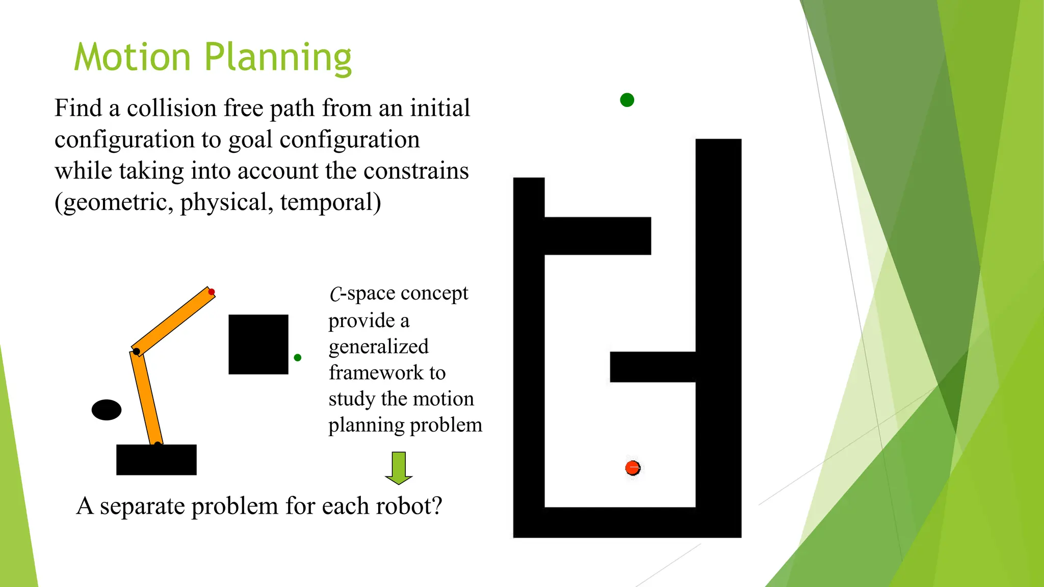
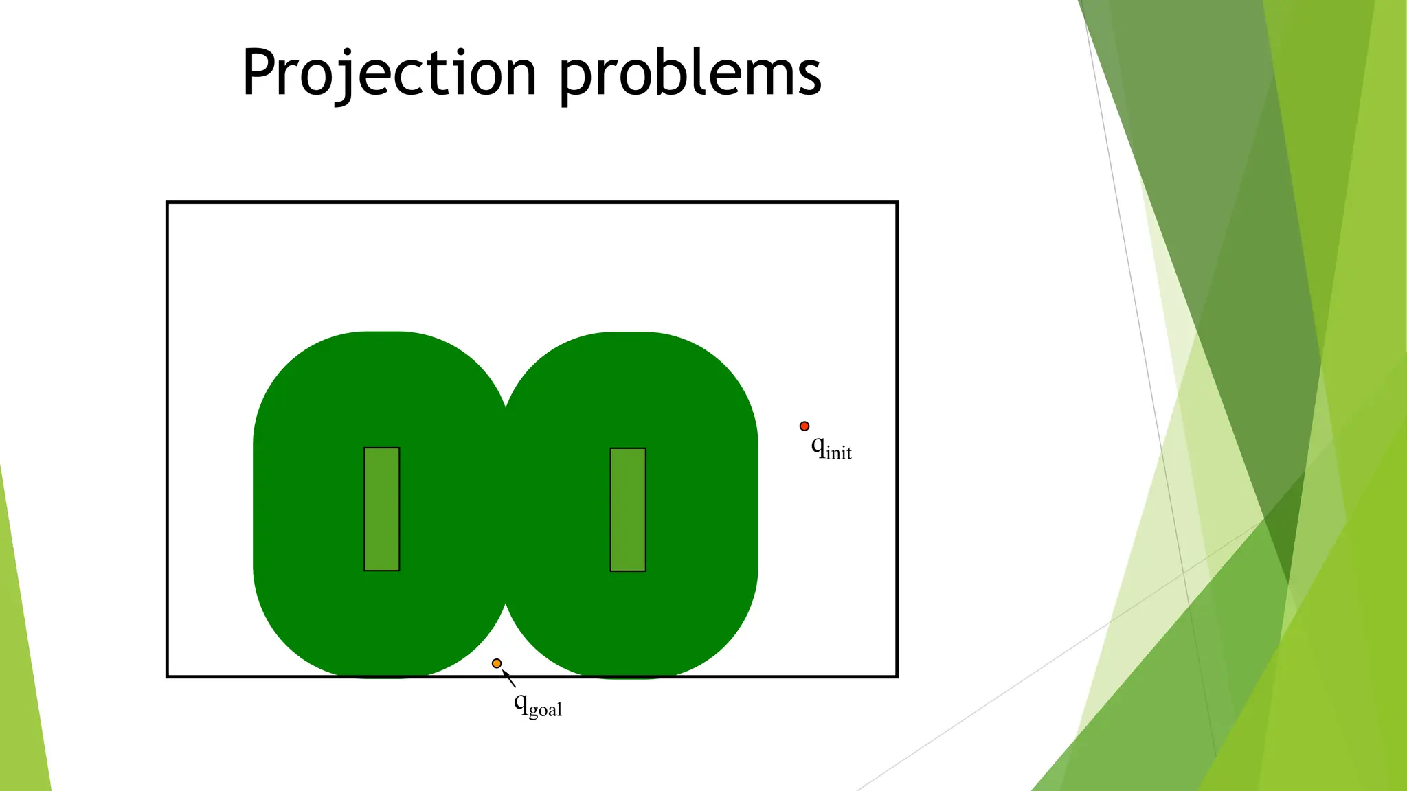
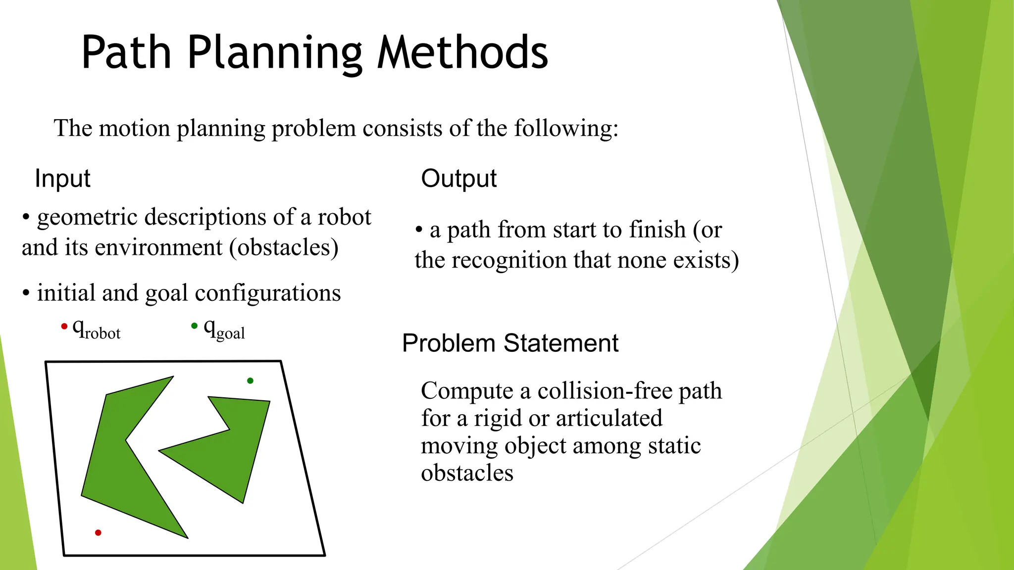
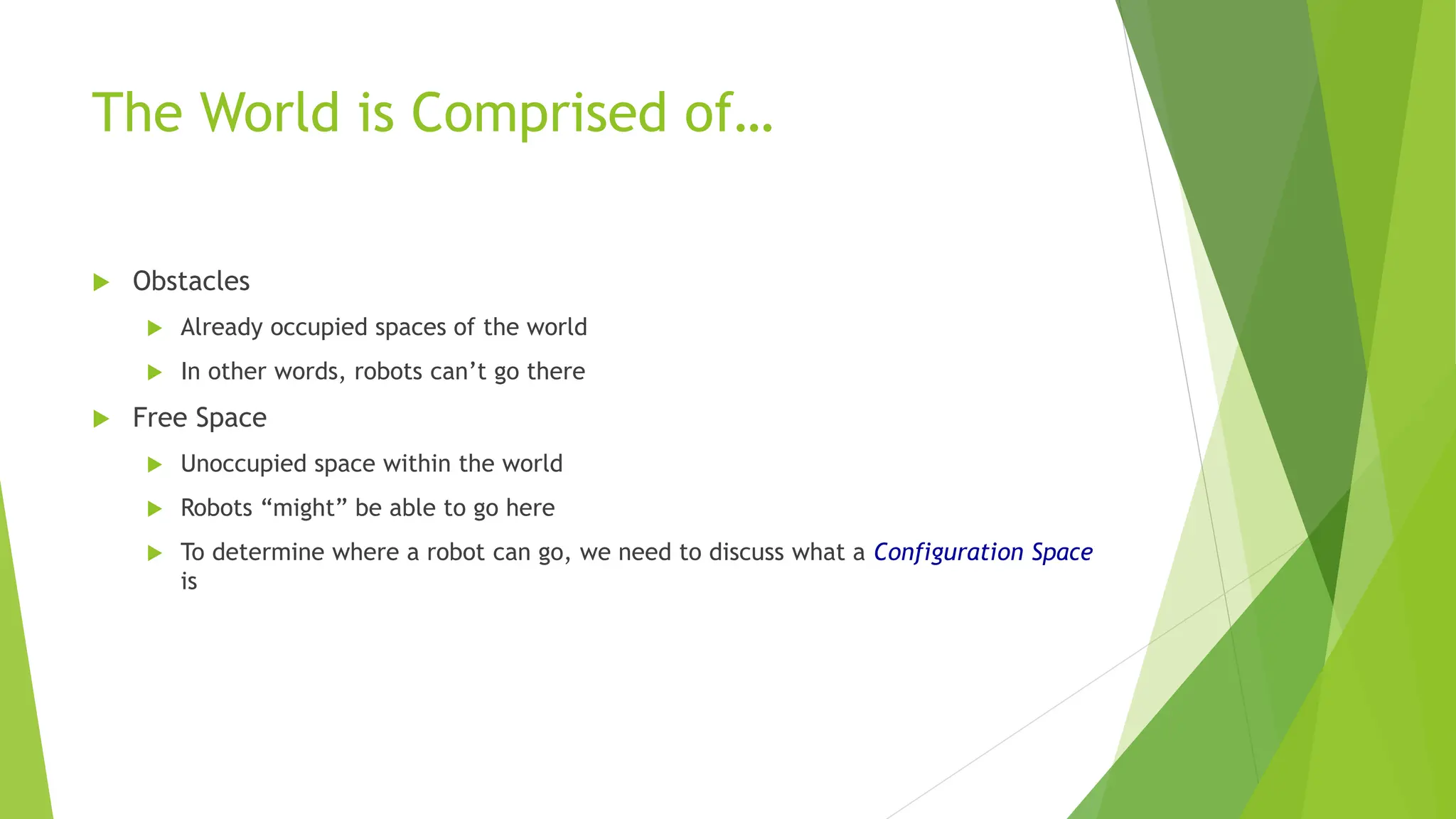
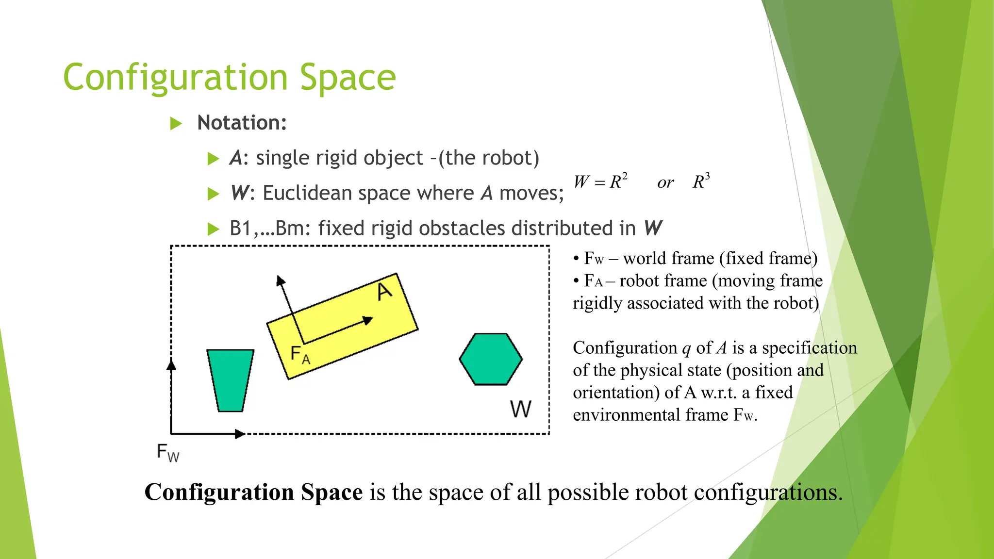
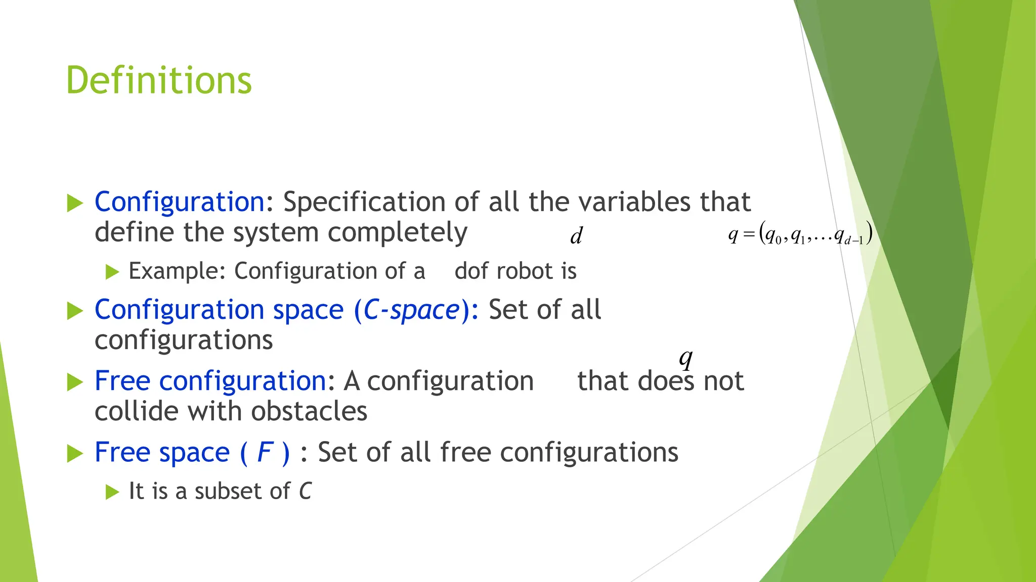
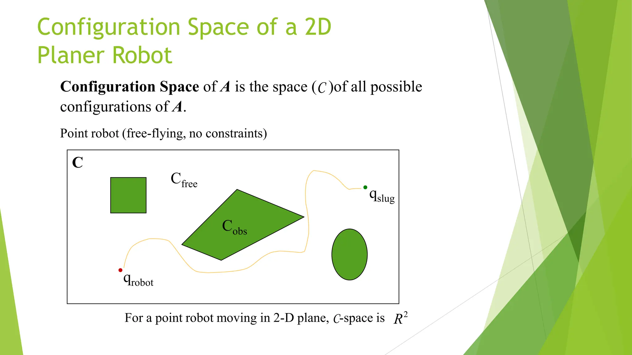
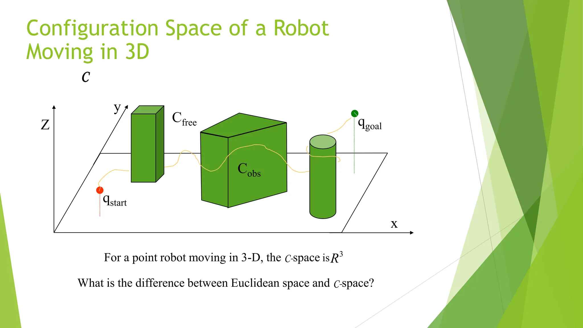
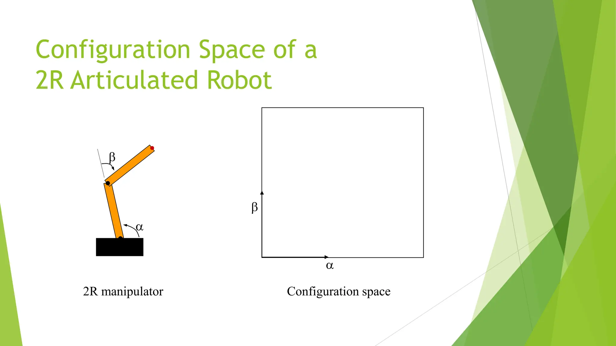
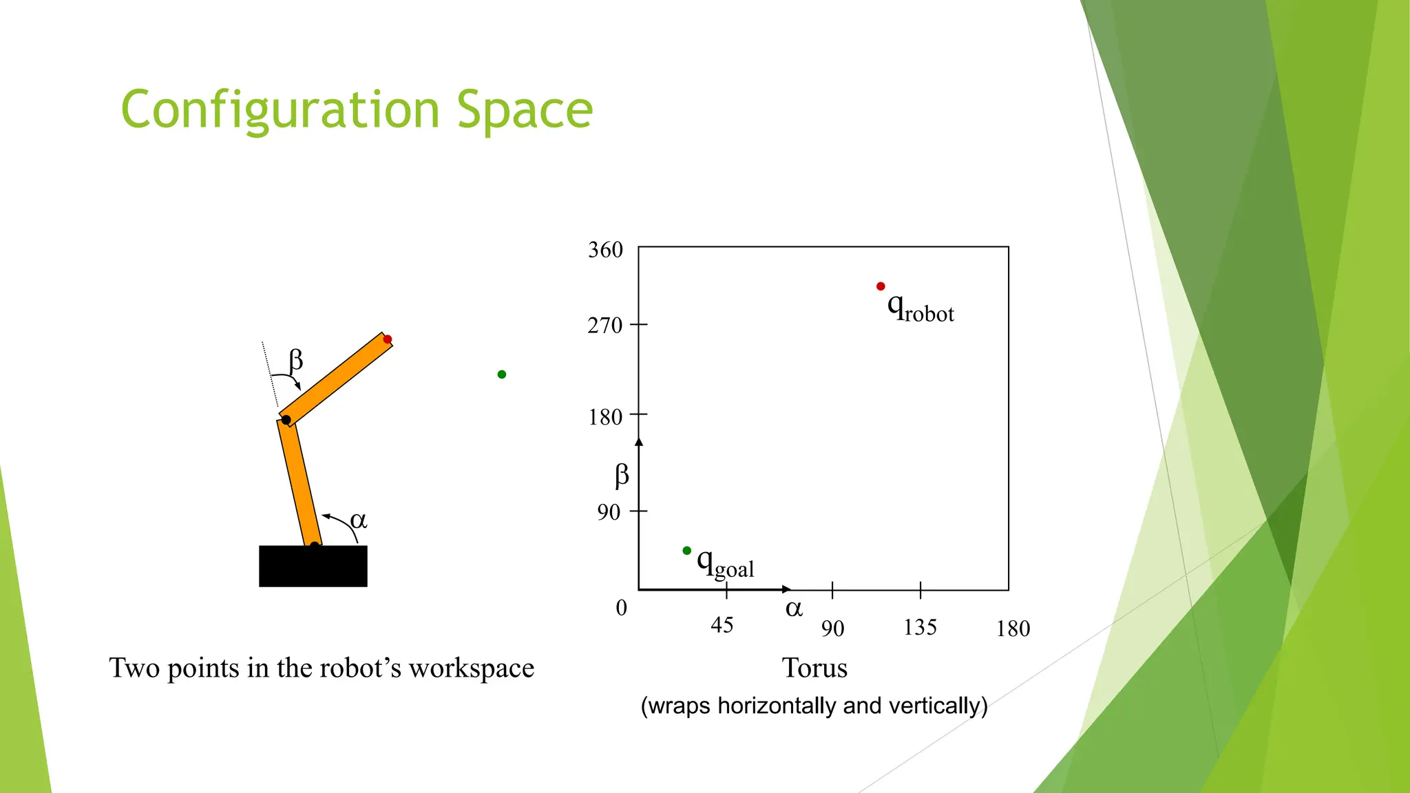
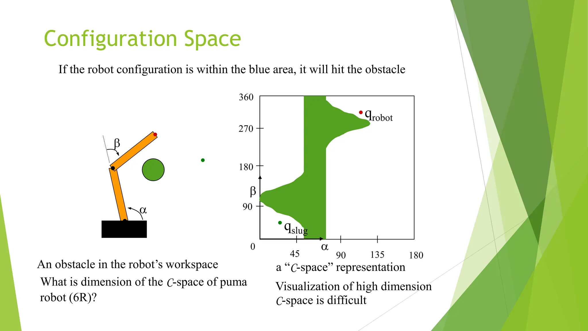
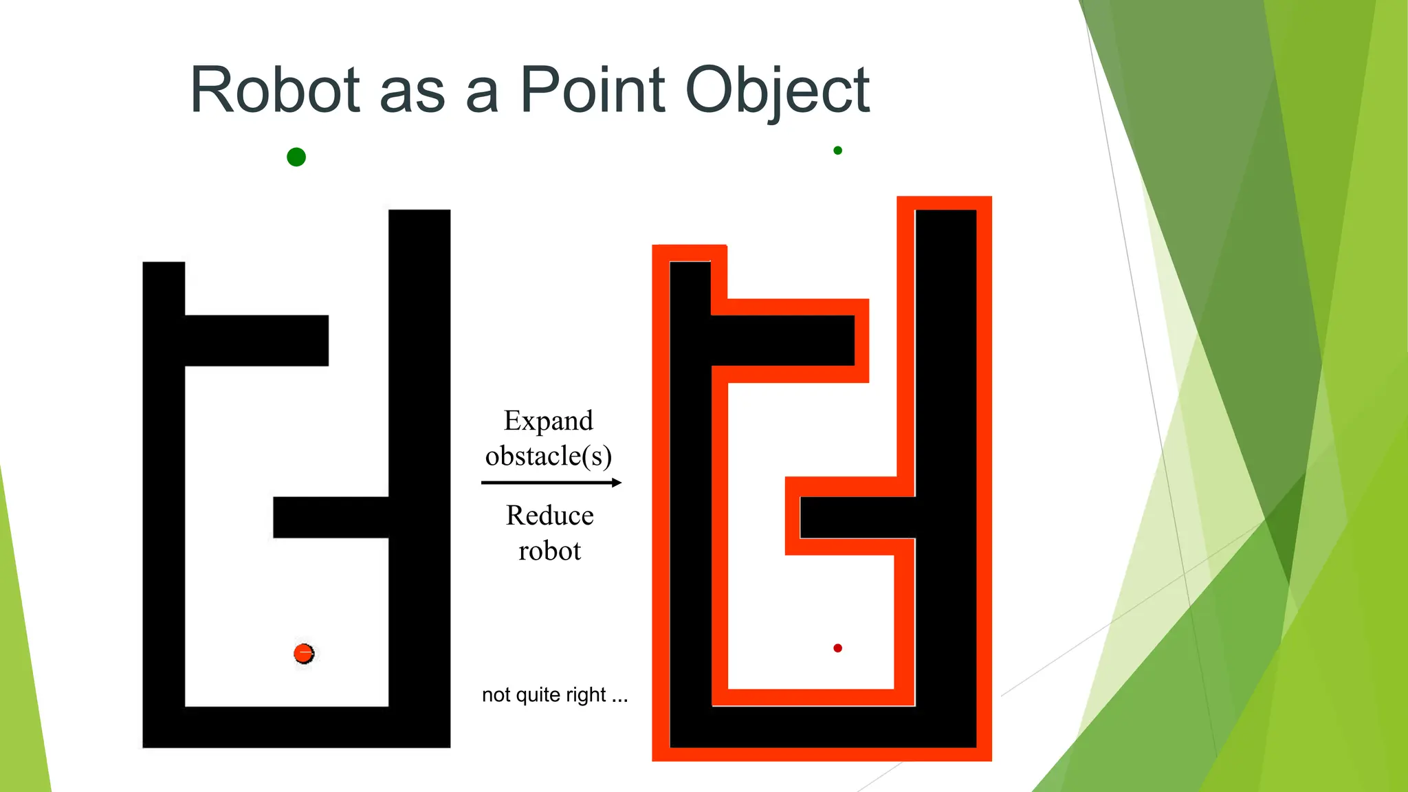
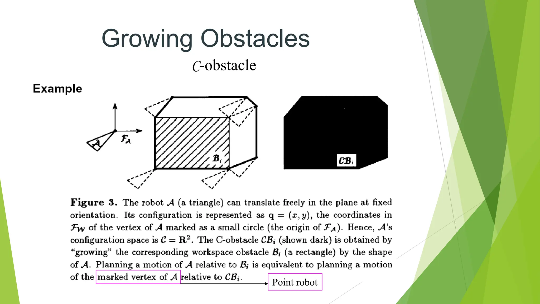
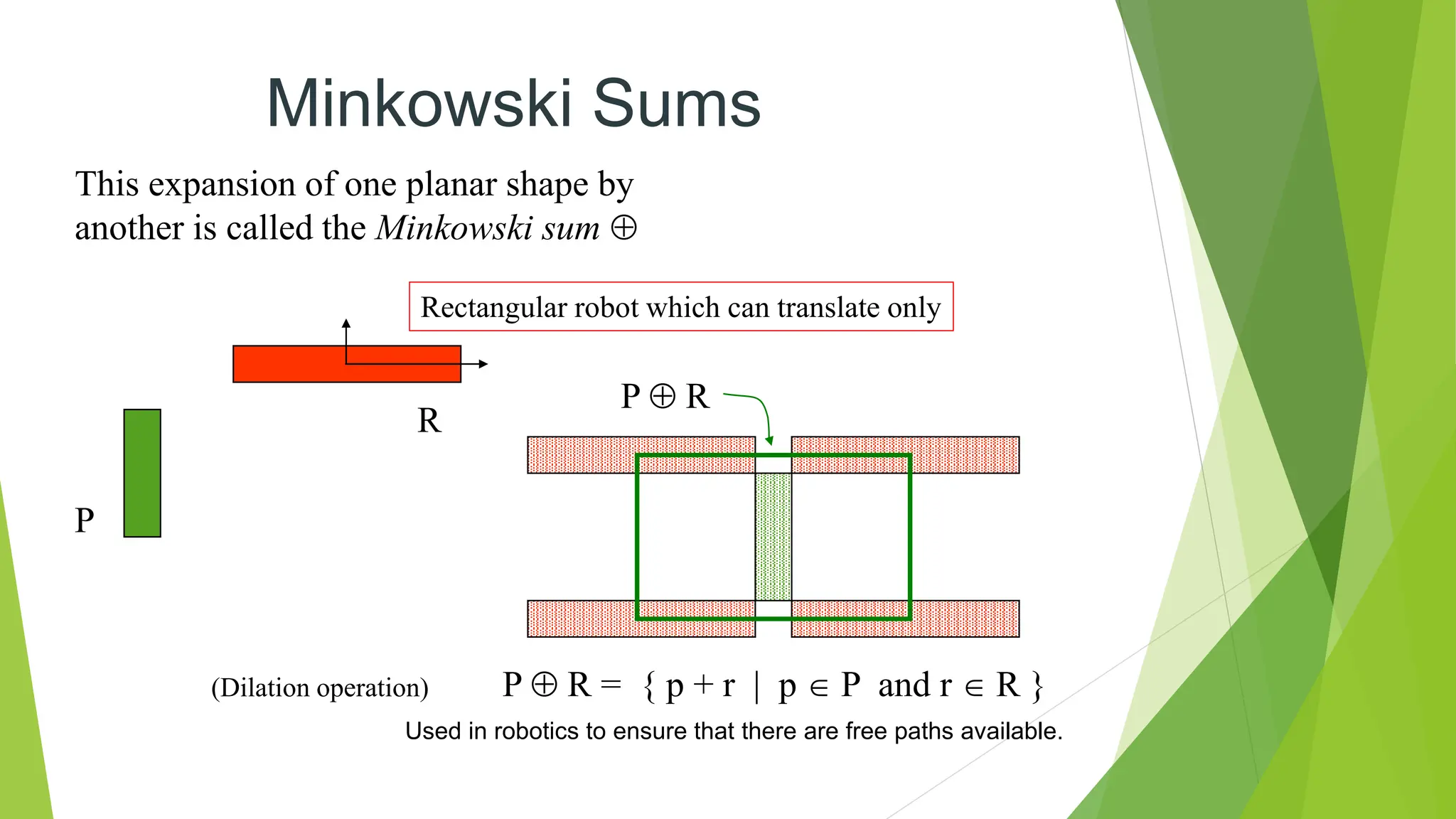
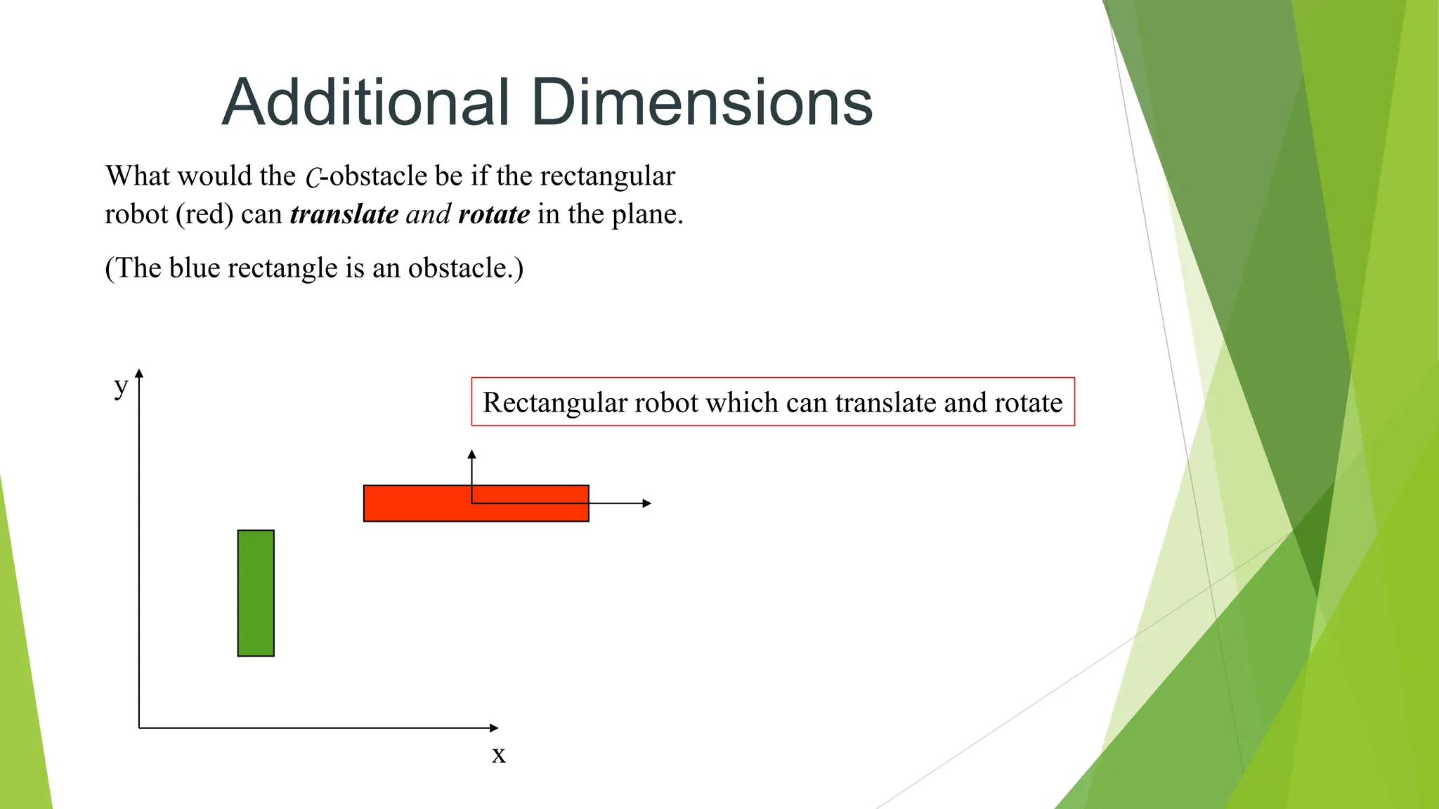
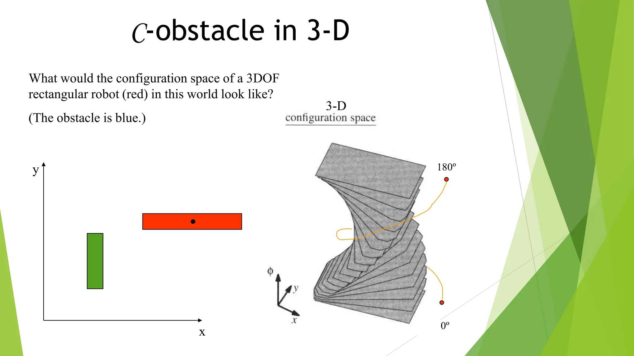
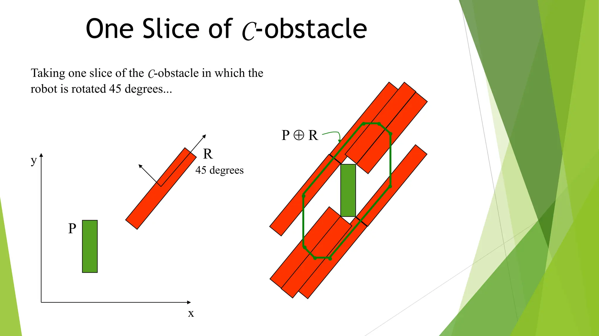
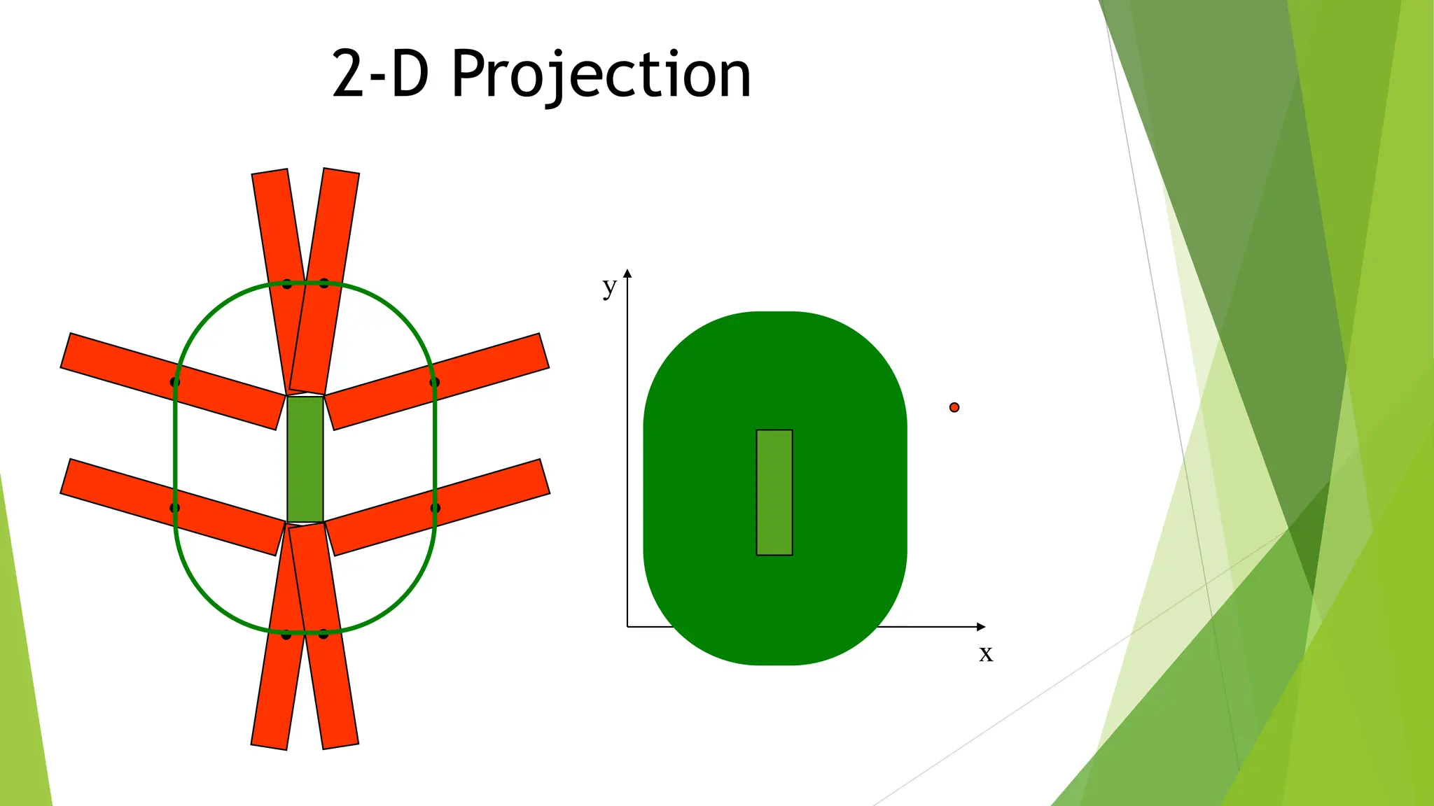
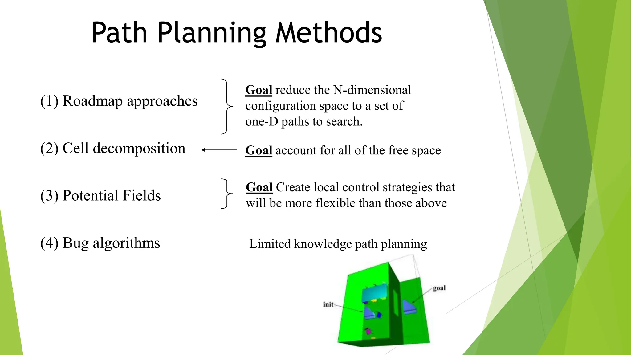
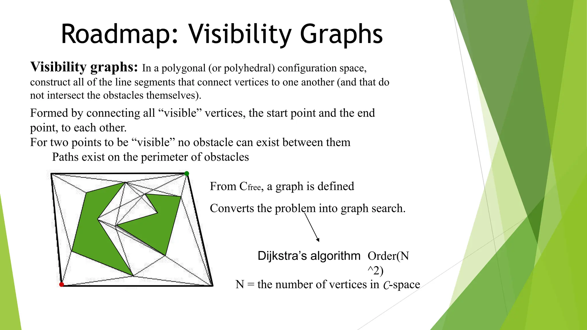
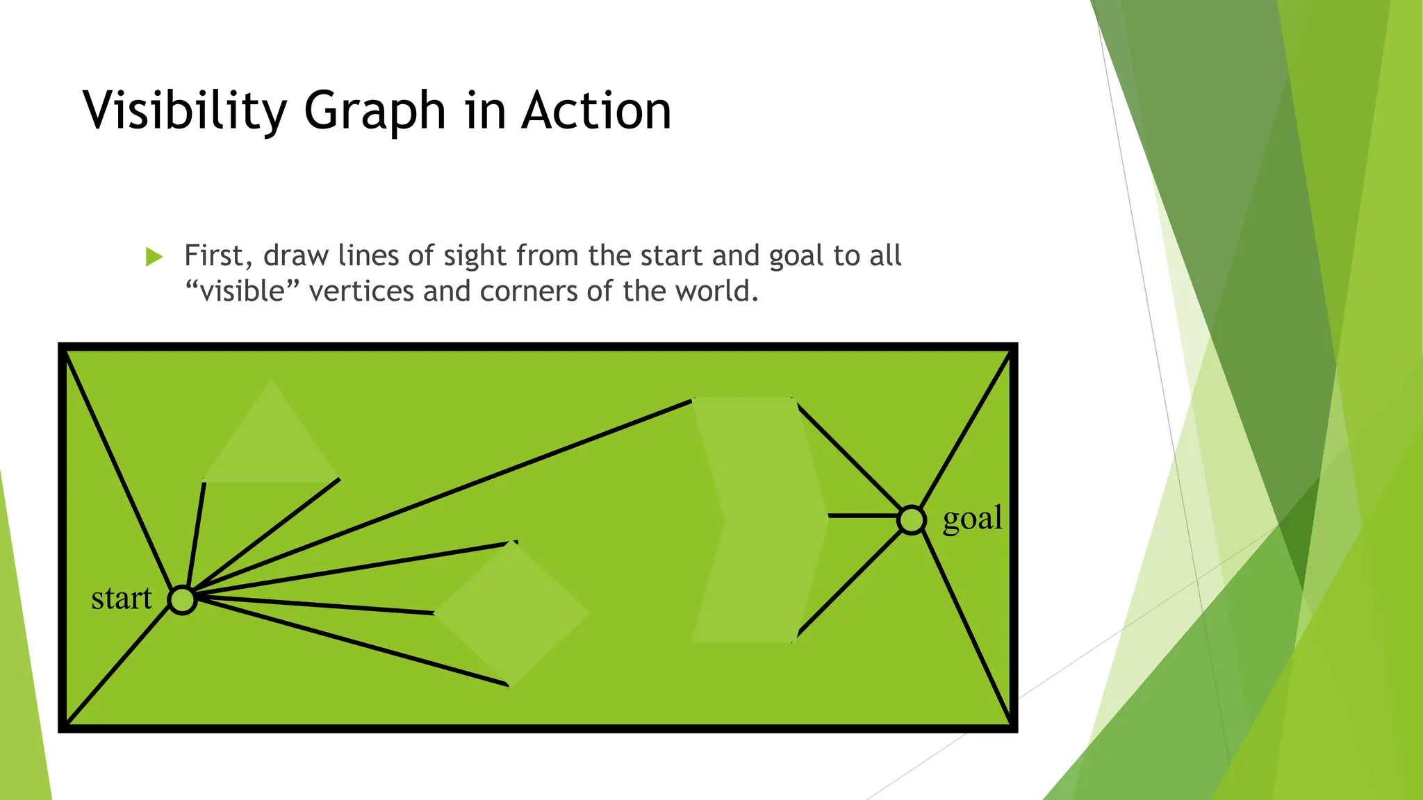
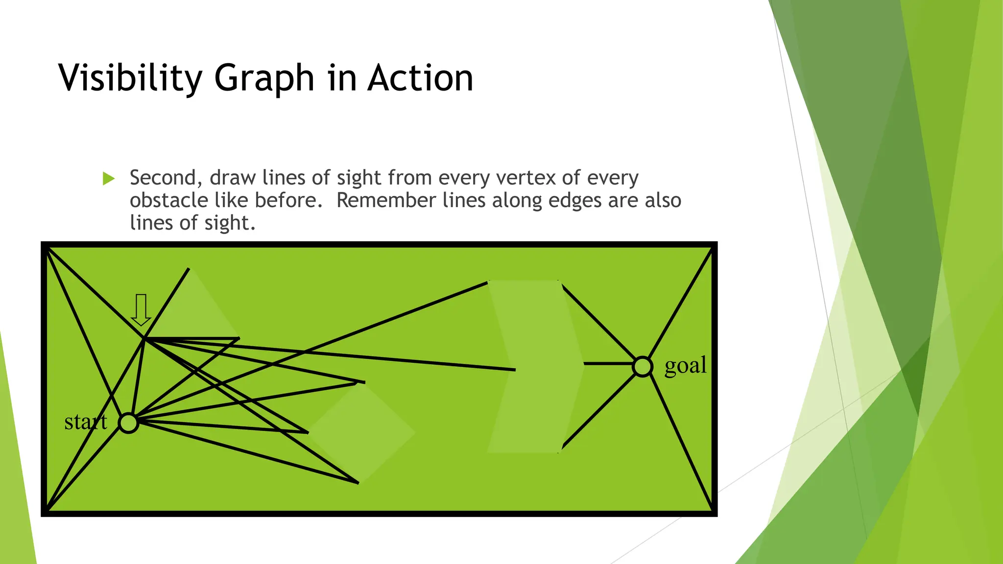
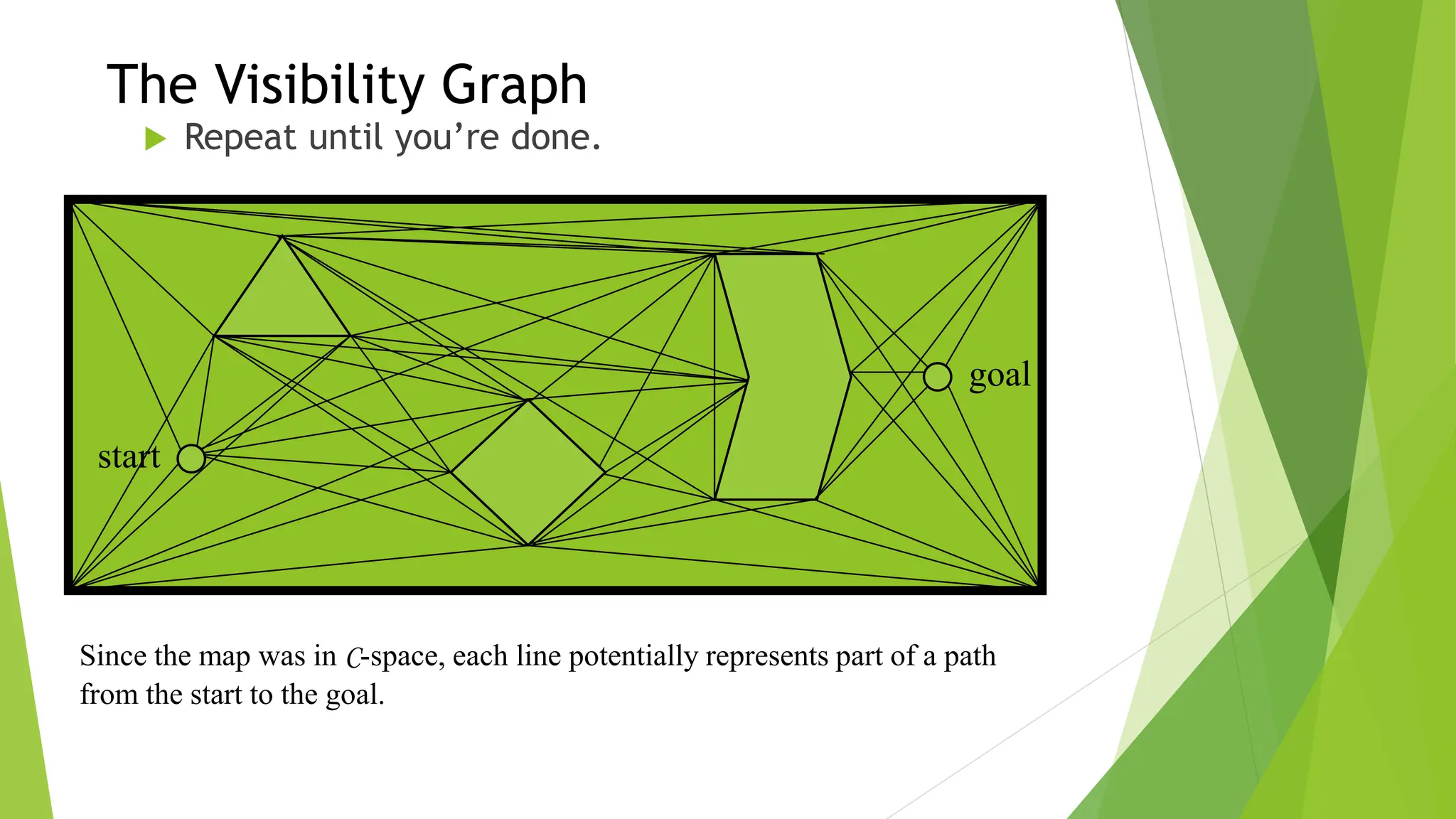
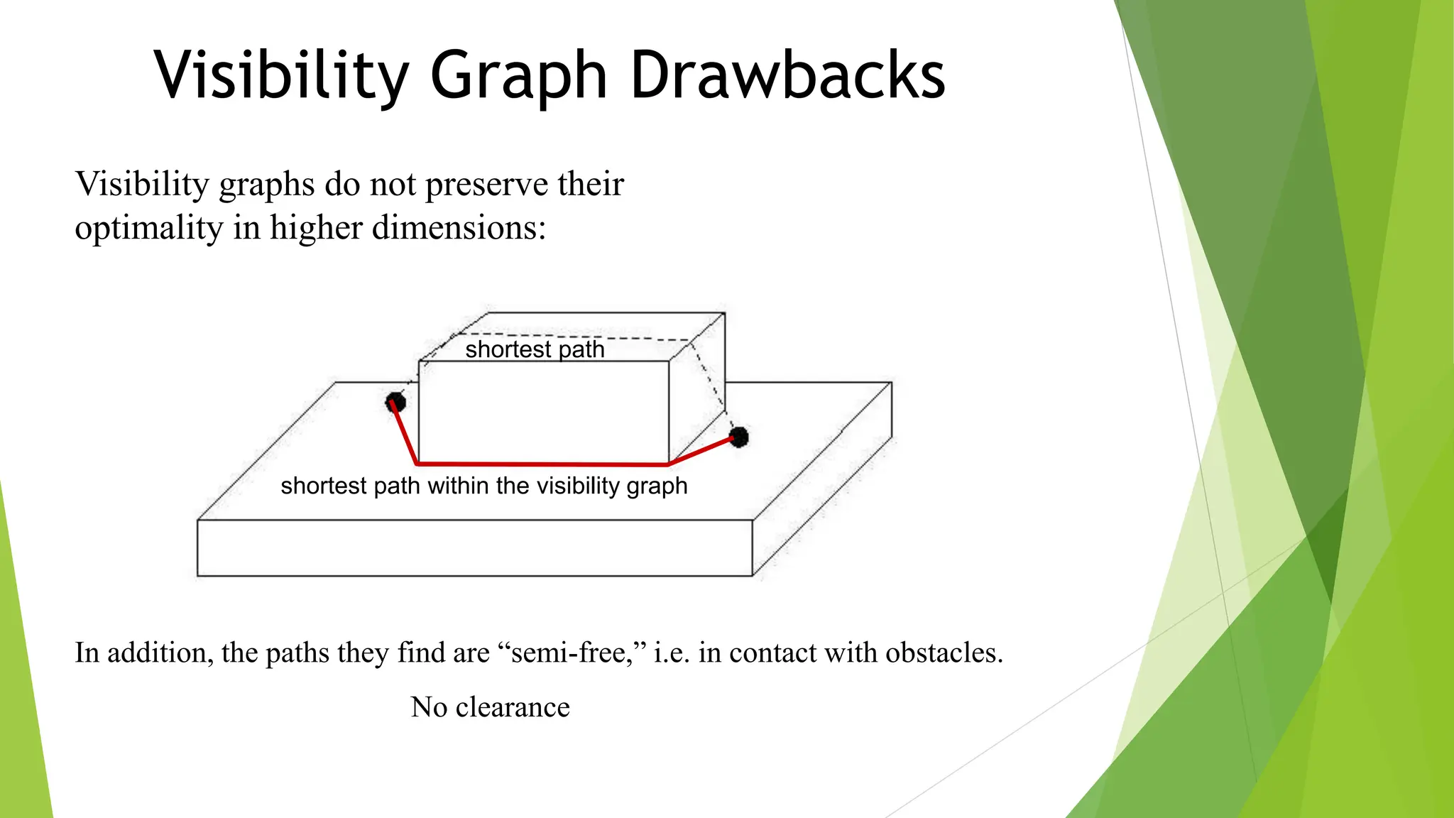
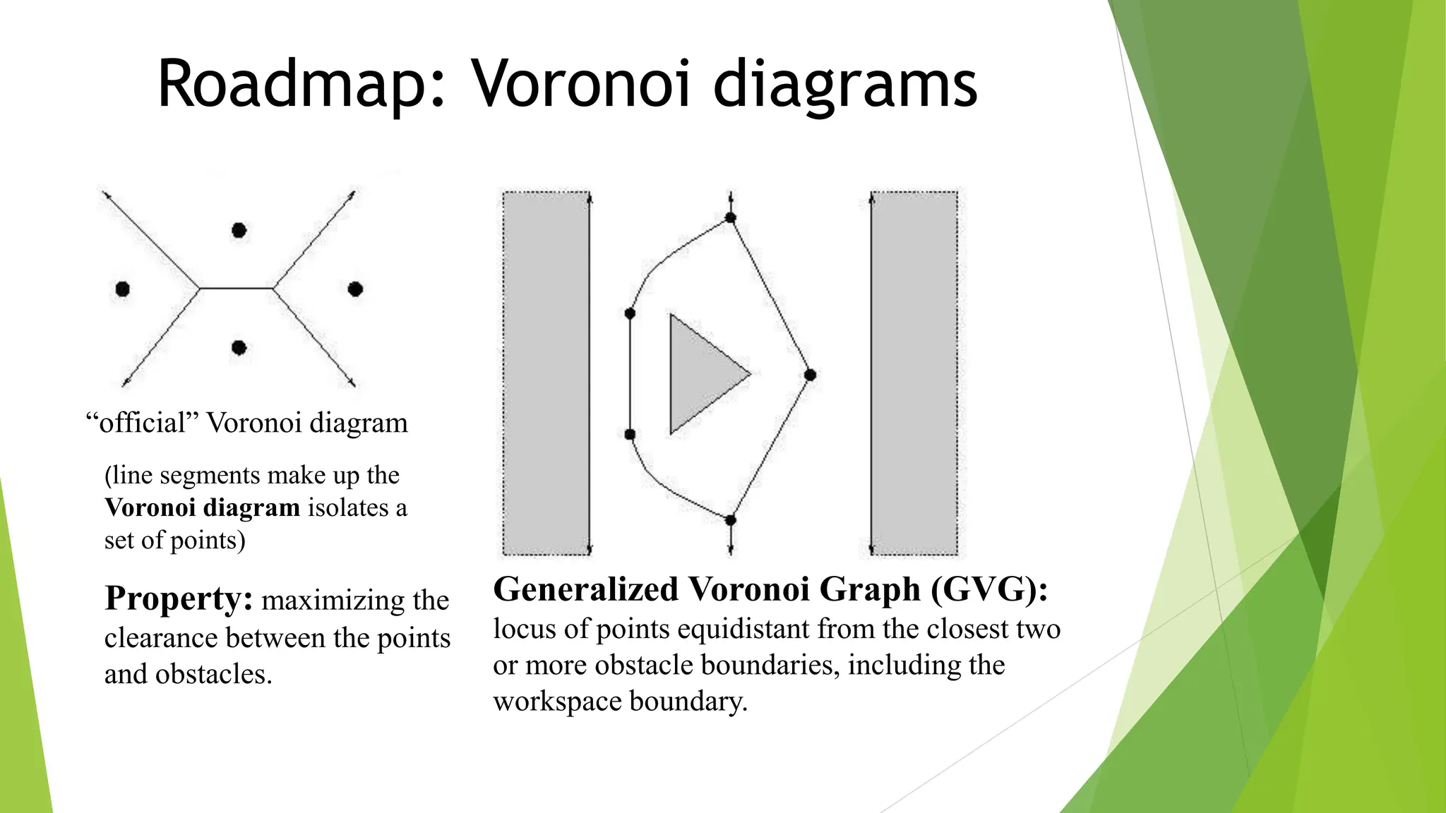
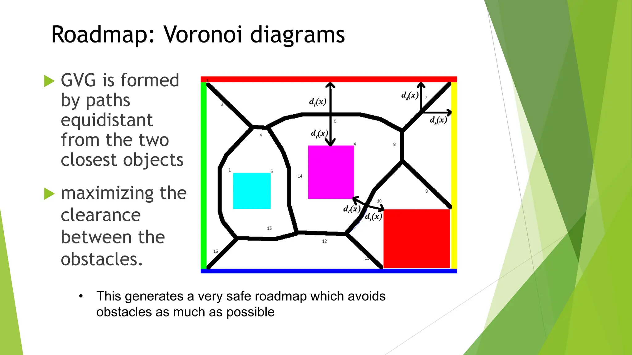
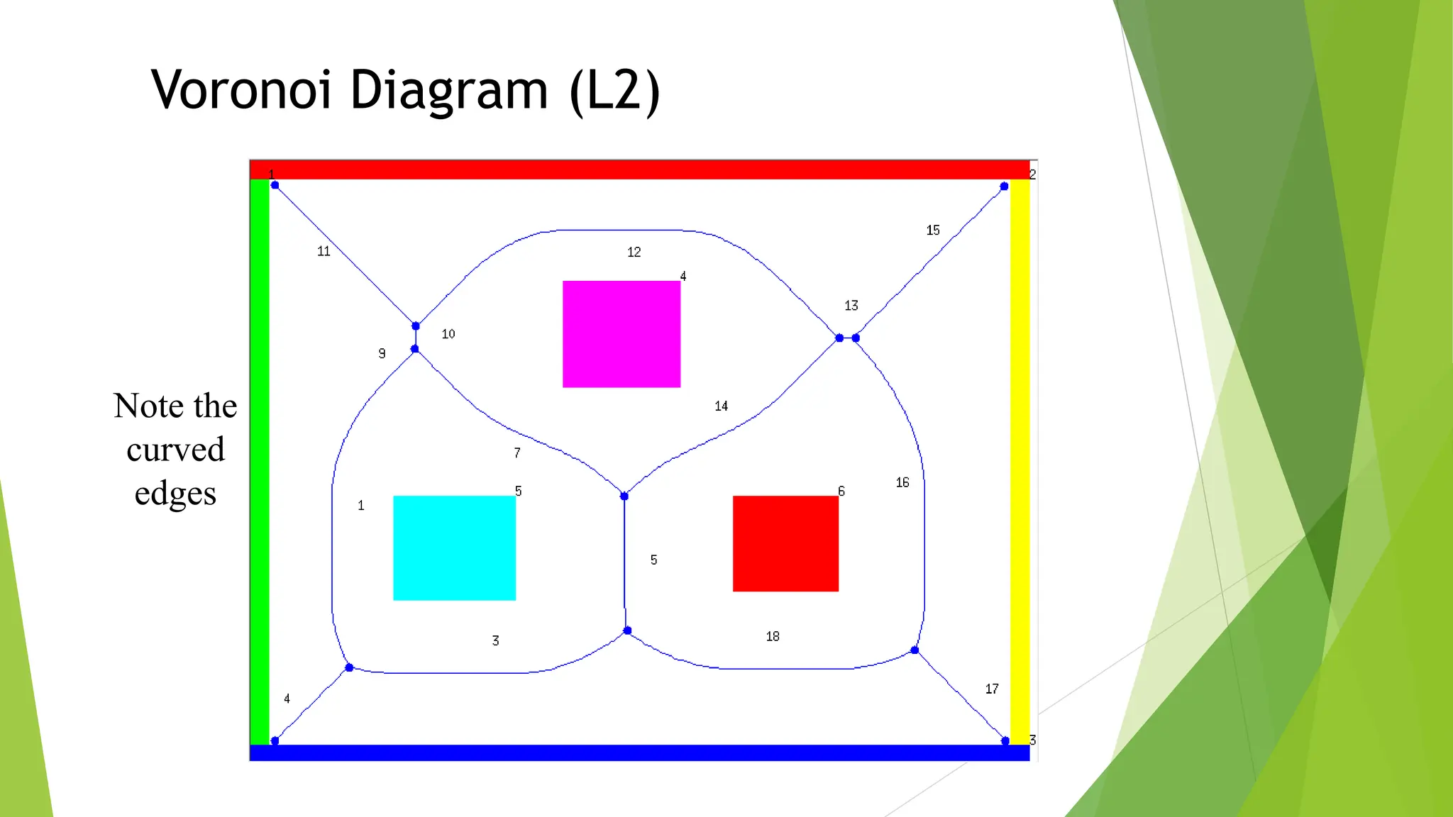
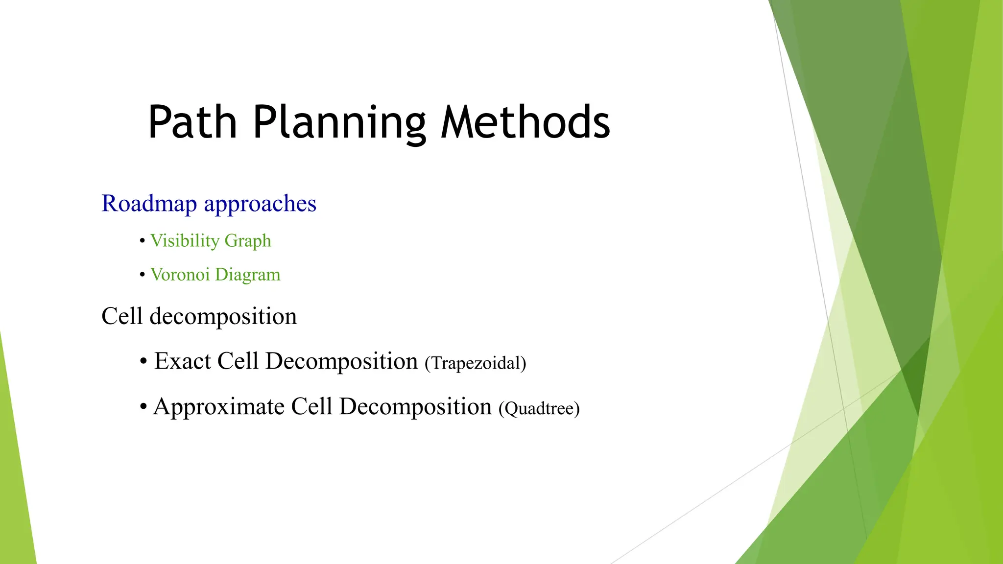
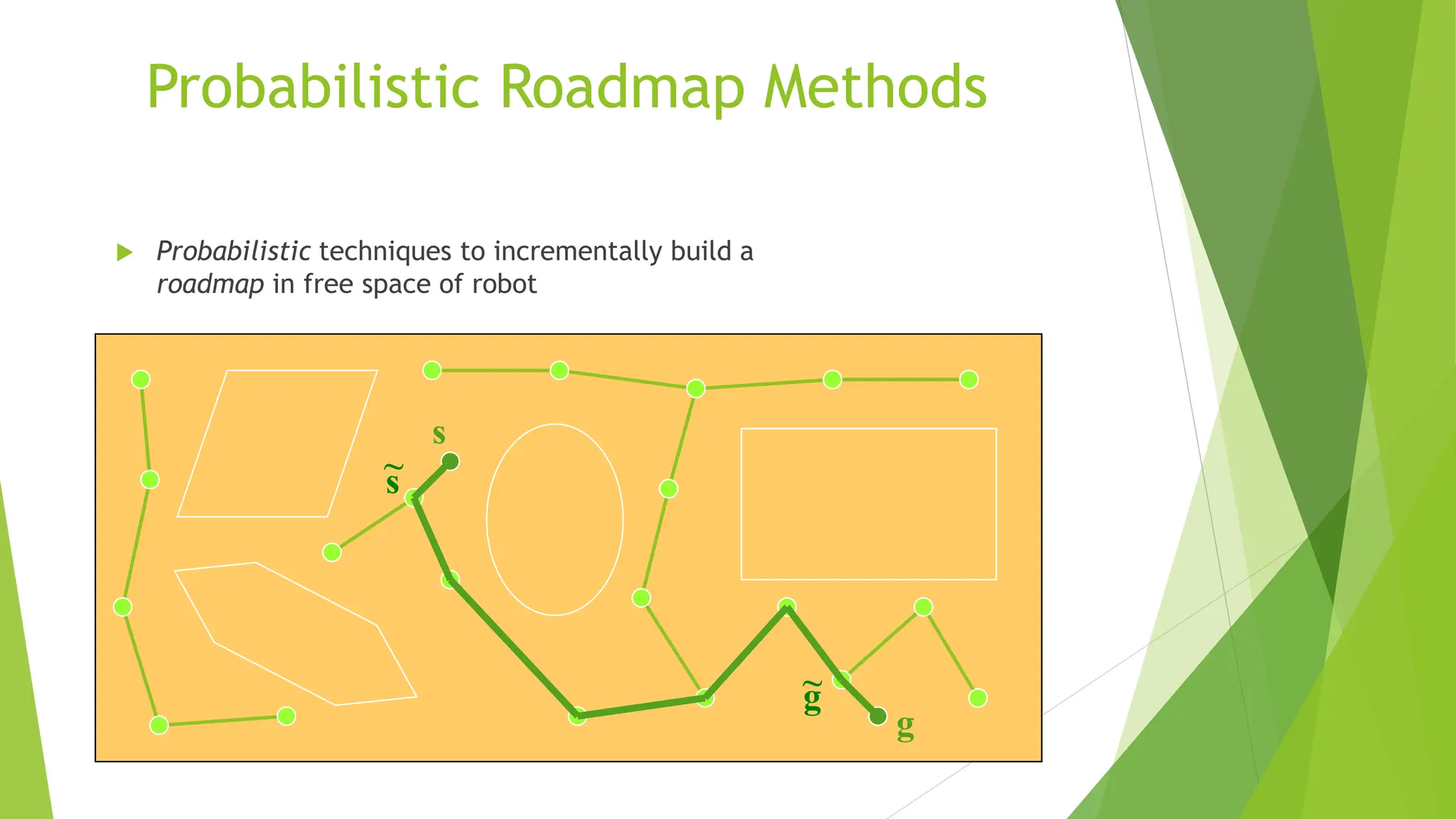
Robot path planning involves generating a collision-free path for a robot to follow between an initial and goal configuration. Key aspects of path planning include: 1) Representing the robot and obstacles in a configuration space (C-space) that accounts for all possible robot states. This allows the path planning problem to be generalized across different robots. 2) Using roadmap approaches like visibility graphs or Voronoi diagrams to reduce the high-dimensional C-space to a graph that can be searched to find paths. 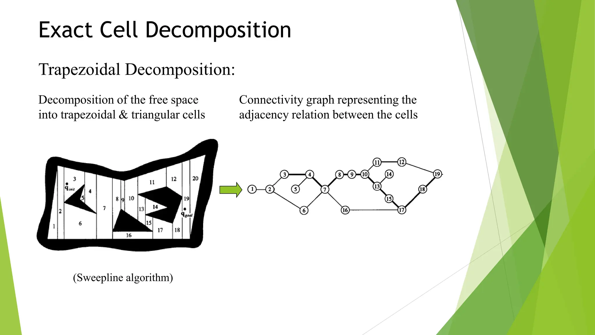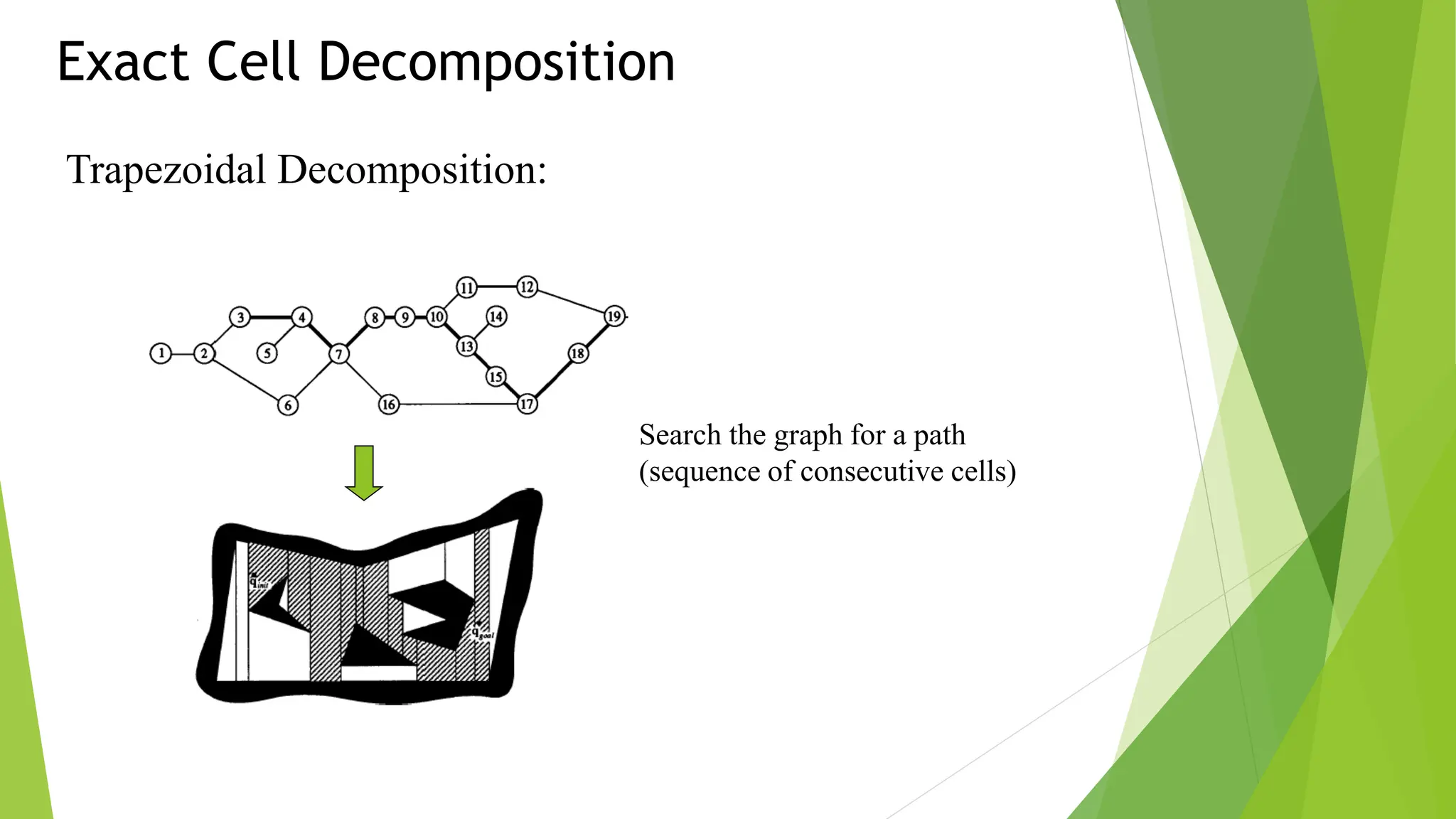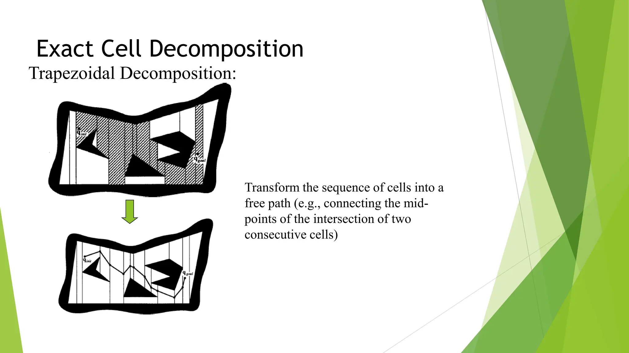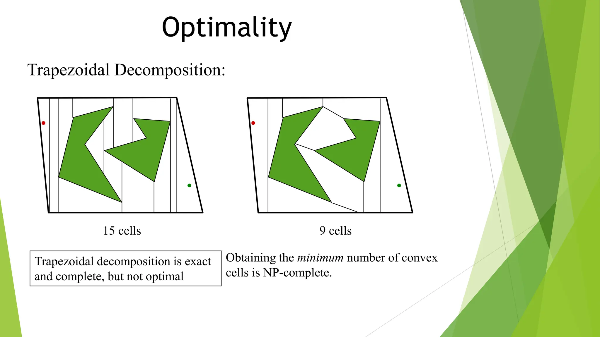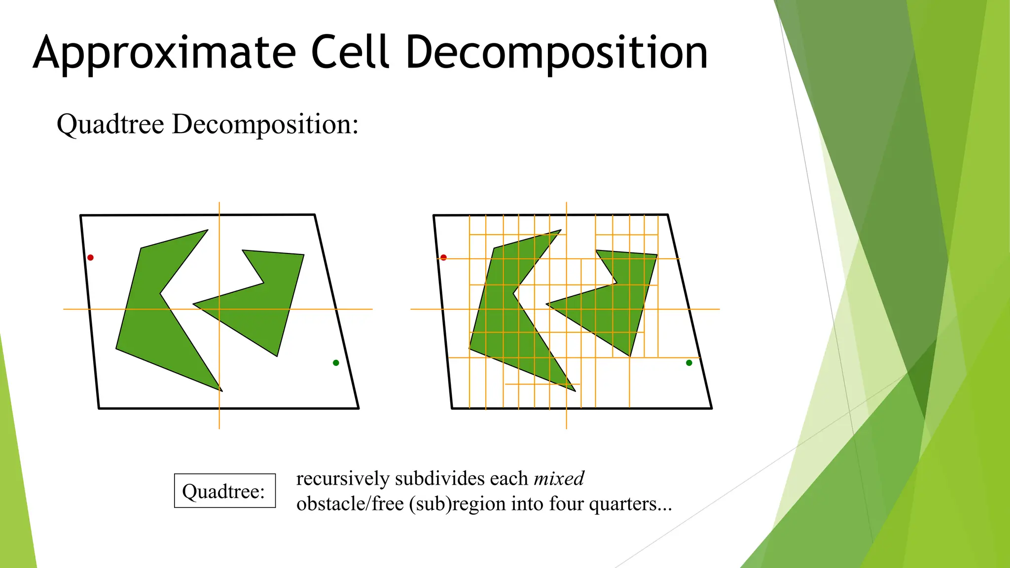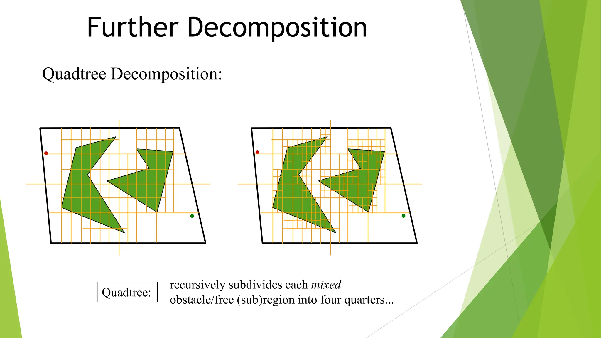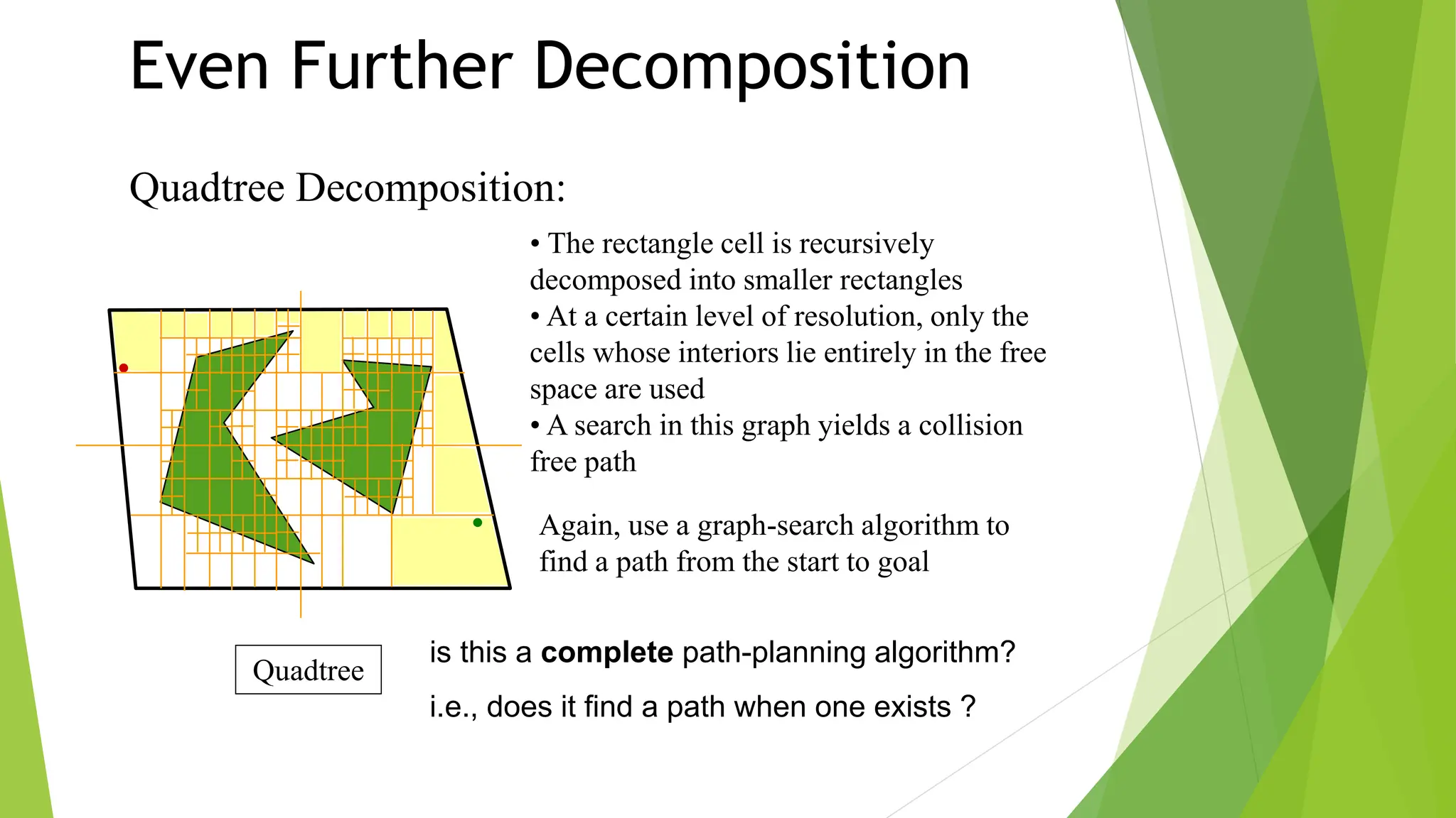3) Cell decomposition methods like trapezoidal decomposition or quadtree decomposition that partition the C-space into simple cells and connect adjacent free cells to form a connectivity graph. 4) Prob

1. Robot path planning,
navigation and localization

2. Robot Motion Planning
Task Plan
Action Plan
Path Plan
Trajectory
Plan
Controller
Sensor
Robot
Tasks
 Path planning
 Geometric path
 Issues: obstacle avoidance, shortest
path
 Trajectory planning,
 “interpolate” or “approximate” the
desired path by a class of polynomial
functions
 Generate a sequence of time-based
“control set points” for the control
of manipulator from the initial
configuration to its destination.

3. The World is Comprised of…
 Obstacles
 Already occupied spaces of the world
 In other words, robots can’t go there
 Free Space
 Unoccupied space within the world
 Robots “might” be able to go here
 To determine where a robot can go, we need to discuss what a Configuration Space
is

4. Configuration Space
 Notation:
 A: single rigid object –(the robot)
 W: Euclidean space where A moves;
 B1,…Bm: fixed rigid obstacles distributed in W
Configuration Space is the space of all possible robot configurations.
3
2
R
or
R
W 
• FW – world frame (fixed frame)
• FA – robot frame (moving frame
rigidly associated with the robot)
Configuration q of A is a specification
of the physical state (position and
orientation) of A w.r.t. a fixed
environmental frame FW.

5. Definitions
 Configuration: Specification of all the variables that
define the system completely
 Example: Configuration of a dof robot is
 Configuration space (C-space): Set of all
configurations
 Free configuration: A configuration that does not
collide with obstacles
 Free space ( F ) : Set of all free configurations
 It is a subset of C
 
1
1
0 ,
, 
 d
q
q
q
q 
d
q

6. Configuration Space of a 2D
Planer Robot
For a point robot moving in 2-D plane, C-space is
Configuration Space of A is the space (C )of all possible
configurations of A.
qslug
qrobot
C
Cfree
Cobs
2
R
Point robot (free-flying, no constraints)

7. Configuration Space of a Robot
Moving in 3D
For a point robot moving in 3-D, the C-space is
Z
x
y
qstart
qgoal
C
Cfree
Cobs
3
R
What is the difference between Euclidean space and C-space?

8. Configuration Space of a
2R Articulated Robot
2R manipulator Configuration space
b
a
b
a

9. Configuration Space
Two points in the robot’s workspace
b
a
270
360
180
90
0
90 180
135
45
Torus
(wraps horizontally and vertically)
qrobot
qgoal
b
a

10. Configuration Space
An obstacle in the robot’s workspace
b
a
270
360
180
90
0
90 180
135
45
qslug
qrobot
a “C-space” representation
b
a
If the robot configuration is within the blue area, it will hit the obstacle
What is dimension of the C-space of puma
robot (6R)?
Visualization of high dimension
C-space is difficult

11. Motion Planning
Find a collision free path from an initial
configuration to goal configuration
while taking into account the constrains
(geometric, physical, temporal)
A separate problem for each robot?
C-space concept
provide a
generalized
framework to
study the motion
planning problem

12. Expand
obstacle(s)
Reduce
robot
not quite right ...
Robot as a Point Object

13. C-obstacle
Point robot
Growing Obstacles

14. This expansion of one planar shape by
another is called the Minkowski sum 
P
R
P  R
Used in robotics to ensure that there are free paths available.
P  R = { p + r | p  P and r  R }
Rectangular robot which can translate only
(Dilation operation)
Minkowski Sums

15. What would the C-obstacle be if the rectangular
robot (red) can translate and rotate in the plane.
(The blue rectangle is an obstacle.)
x
y
Rectangular robot which can translate and rotate
Additional Dimensions

16. C-obstacle in 3-D
What would the configuration space of a 3DOF
rectangular robot (red) in this world look like?
(The obstacle is blue.)
x
y
0º
180º
3-D

17. One Slice of C-obstacle
Taking one slice of the C-obstacle in which the
robot is rotated 45 degrees...
x
y
45 degrees
P
R
P  R

18. 2-D Projection
x
y

19. Projection problems
qinit
qgoal

20. Path Planning Methods
The motion planning problem consists of the following:
Input Output
• geometric descriptions of a robot
and its environment (obstacles)
• initial and goal configurations
• a path from start to finish (or
the recognition that none exists)
qgoal
qrobot
Problem Statement
Compute a collision-free path
for a rigid or articulated
moving object among static
obstacles

21. Path Planning Methods
(1) Roadmap approaches
(2) Cell decomposition
(3) Potential Fields
(4) Bug algorithms
Goal reduce the N-dimensional
configuration space to a set of
one-D paths to search.
Goal account for all of the free space
Goal Create local control strategies that
will be more flexible than those above
Limited knowledge path planning

22. Roadmap: Visibility Graphs
Visibility graphs: In a polygonal (or polyhedral) configuration space,
construct all of the line segments that connect vertices to one another (and that do
not intersect the obstacles themselves).
From Cfree, a graph is defined
Converts the problem into graph search.
Dijkstra’s algorithm Order(N
^2)
N = the number of vertices in C-space
Formed by connecting all “visible” vertices, the start point and the end
point, to each other.
For two points to be “visible” no obstacle can exist between them
Paths exist on the perimeter of obstacles

23. Visibility Graph in Action
 First, draw lines of sight from the start and goal to all
“visible” vertices and corners of the world.
start
goal

24. Visibility Graph in Action
 Second, draw lines of sight from every vertex of every
obstacle like before. Remember lines along edges are also
lines of sight.
start
goal

25. The Visibility Graph
 Repeat until you’re done.
start
goal
Since the map was in C-space, each line potentially represents part of a path
from the start to the goal.

26. Visibility Graph Drawbacks
Visibility graphs do not preserve their
optimality in higher dimensions:
In addition, the paths they find are “semi-free,” i.e. in contact with obstacles.
shortest path
shortest path within the visibility graph
No clearance

27. “official” Voronoi diagram
(line segments make up the
Voronoi diagram isolates a
set of points)
Roadmap: Voronoi diagrams
Generalized Voronoi Graph (GVG):
locus of points equidistant from the closest two
or more obstacle boundaries, including the
workspace boundary.
Property: maximizing the
clearance between the points
and obstacles.

28. Roadmap: Voronoi diagrams
 GVG is formed
by paths
equidistant
from the two
closest objects
 maximizing the
clearance
between the
obstacles.
• This generates a very safe roadmap which avoids
obstacles as much as possible

29. Voronoi Diagram: Metrics
• Many ways to measure distance; two are:
– L1 metric
• (x,y) : |x| + |y| = const
– L2 metric
• (x,y) : x2 +y2 = const

30. Voronoi Diagram (L1)
Note the
lack of
curved
edges

31. Voronoi Diagram (L2)
Note the
curved
edges

32. Path Planning Methods
Roadmap approaches
• Visibility Graph
• Voronoi Diagram
Cell decomposition
• Exact Cell Decomposition (Trapezoidal)
• Approximate Cell Decomposition (Quadtree)

33. Exact Cell Decomposition
Decomposition of the free space
into trapezoidal & triangular cells
Connectivity graph representing the
adjacency relation between the cells
(Sweepline algorithm)
Trapezoidal Decomposition:

34. Exact Cell Decomposition
Search the graph for a path
(sequence of consecutive cells)
Trapezoidal Decomposition:

35. Exact Cell Decomposition
Transform the sequence of cells into a
free path (e.g., connecting the mid-
points of the intersection of two
consecutive cells)
Trapezoidal Decomposition:

36. Obtaining the minimum number of convex
cells is NP-complete.
Optimality
15 cells 9 cells
Trapezoidal decomposition is exact
and complete, but not optimal
Trapezoidal Decomposition:

37. Quadtree Decomposition:
Approximate Cell Decomposition
recursively subdivides each mixed
obstacle/free (sub)region into four quarters...
Quadtree:

38. Further Decomposition
recursively subdivides each mixed
obstacle/free (sub)region into four quarters...
Quadtree:
Quadtree Decomposition:

39. Even Further Decomposition
Again, use a graph-search algorithm to
find a path from the start to goal
Quadtree
is this a complete path-planning algorithm?
i.e., does it find a path when one exists ?
Quadtree Decomposition:
• The rectangle cell is recursively
decomposed into smaller rectangles
• At a certain level of resolution, only the
cells whose interiors lie entirely in the free
space are used
• A search in this graph yields a collision
free path

40. Probablistic Roadmap Methods
 What is a PRM (Probablistic Roadmap Method)
 A probabilistic road map is a discrete representation of a
continuous configuration space generated by randomly
sampling the free configurations of the C-space and
connecting those points into a graph
 Complete path planning in high dimensional C- spaces
is very complex
 PRM methods boost performance by trading
completeness for probabilistic completeness
 Two phase approach: Learning phase, Query phase

41. Probabilistic Roadmap Methods
 Probabilistic techniques to incrementally build a
roadmap in free space of robot
• Efficiency-driven
• Robots with many dofs (high-dim C-
spaces)
• Static environments
s
g
s
~
g
~

42. Learning Phase
 Learning phase:
 Construction:
 randomly sample free space and create a list of nodes in free space.
 Connect all the nearest neighbors using a fast local planner.
 Store the graph whose nodes are configurations and edges are paths computed by local
planner
 Expansion step: Find “Difficult” nodes and expand the graph around them using
random walk techniques

43. Query Phase
 Find a path from the start and goal positions to two nodes of the roadmap
 Search the graph to find a sequence of edges connecting those nodes in the
roadmap
 Concatenating successive segments gives a feasible path for robot.

44. Thank You
Any Questions?