The document discusses risk-aversion and risk-premium through the lens of utility theory, particularly using examples like a coin flip game. It emphasizes the relationship between outcome variance, personal risk-aversion, and the formulation of a utility function that captures these aspects. The analysis includes mathematical formulations for absolute and relative risk-premiums in the context of constant absolute and relative risk-aversion utilities.

1. Understanding Risk-Aversion through Utility Theory
Ashwin Rao
ICME, Stanford University
November 12, 2018
Ashwin Rao (Stanford) Utility Theory November 12, 2018 1 / 13

2. Intuition on Risk-Aversion and Risk-Premium
Game where your payoff is based on outcome of a fair coin
You get $100 for HEAD and $0 for TAIL
How much would you pay to play this game?
You immediately say: “Of course, $50”
Then you think a bit, and say: “A little less than $50”
Less because you want to “be compensated for taking the risk”
The word Risk refers to the degree of variation of the outcome
We call this risk-compensation as Risk-Premium
Our personality-based degree of risk fear is known as Risk-Aversion
So, we end up paying $50 minus Risk-Premium to play the game
Risk-Premium grows with Outcome-Variance & Risk-Aversion
Ashwin Rao (Stanford) Utility Theory November 12, 2018 2 / 13

3. Specifying Risk-Aversion through a Utility function
So the amount we’d pay to consume a random outcome involves
The Mean of the outcome (often called Reward)
The Variance of the outcome (Risk)
Our personal degree of Risk-Aversion
More generally, we want a “valuation formula” that combines:
The entire probability distribution of the random outcome
A function of the outcome that captures our Risk-Aversion
This function of the outcome is called Utility (denoted U)
It relates to a fundamental concept called Utility of Consumption
We will illustrate this economic concept with a real-life example
Ashwin Rao (Stanford) Utility Theory November 12, 2018 3 / 13

4. Law of Diminishing Marginal Utility
Ashwin Rao (Stanford) Utility Theory November 12, 2018 4 / 13

5. Utility of Consumption and Certainty-Equivalent Value
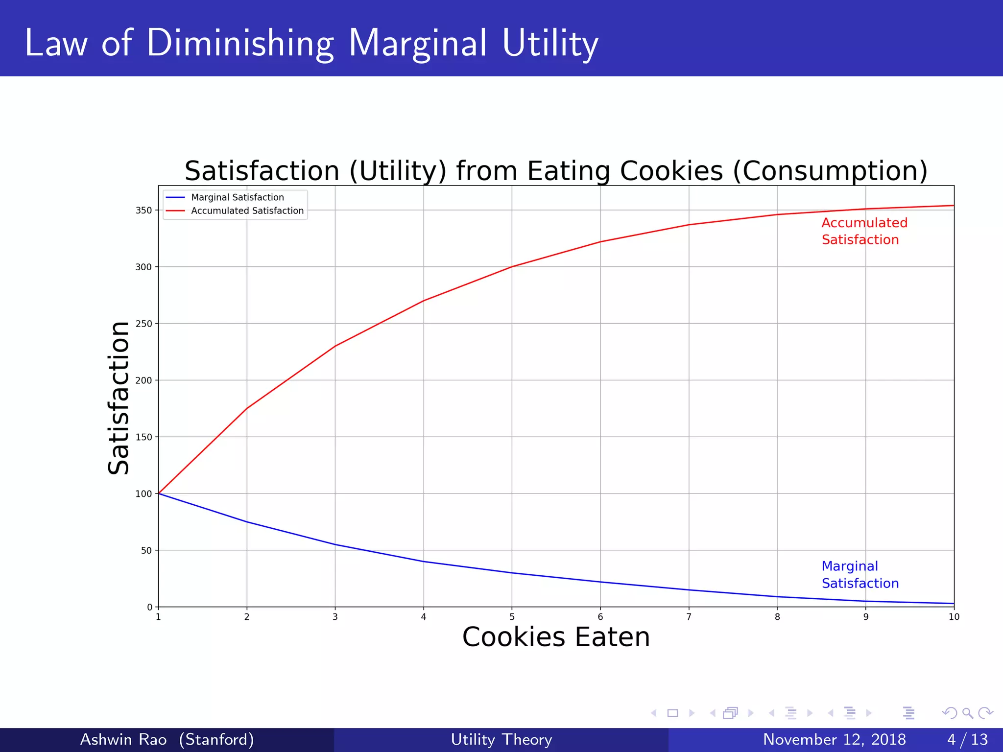
Marginal Satisfaction of eating cookies is a diminishing function
Hence, Accumulated Satisfaction is a concave function
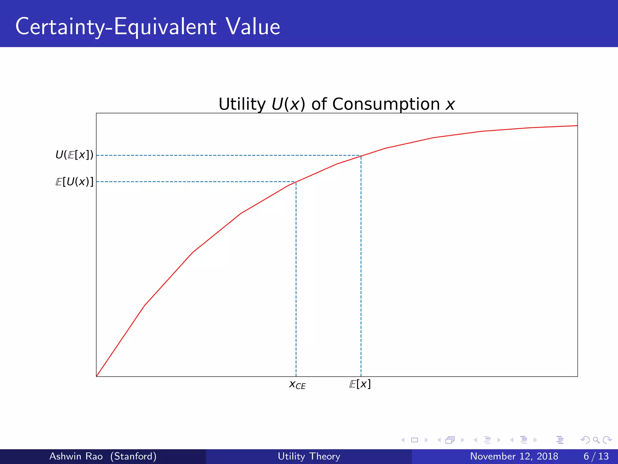
Accumulated Satisfaction represents Utility of Consumption U(x)
Where x represents the uncertain outcome being consumed
Degree of concavity represents extent of our Risk-Aversion
Concave U(·) function ⇒ E[U(x)] < U(E[x])
We define Certainty-Equivalent Value xCE = U−1(E[U(x)])
Denotes certain amount we’d pay to consume an uncertain outcome
Absolute Risk-Premium πA = E[x] − xCE
Relative Risk-Premium πR = πA
E[x] = E[x]−xCE
E[x] = 1 − xCE
E[x]
Ashwin Rao (Stanford) Utility Theory November 12, 2018 5 / 13

6. Certainty-Equivalent Value
Ashwin Rao (Stanford) Utility Theory November 12, 2018 6 / 13

7. Calculating the Risk-Premium
We develop mathematical formalism to calculate Risk-Premia πA, πR
To lighten notation, we refer to E[x] as ¯x and Variance of x as σ2
x
Taylor-expand U(x) around ¯x, ignoring terms beyond quadratic
U(x) ≈ U(¯x) + U (¯x) · (x − ¯x) +
1
2
U (¯x) · (x − ¯x)2
Taylor-expand U(xCE ) around ¯x, ignoring terms beyond linear
U(xCE ) ≈ U(¯x) + U (¯x) · (xCE − ¯x)
Taking the expectation of the U(x) expansion, we get:
E[U(x)] ≈ U(¯x) +
1
2
· U (¯x) · σ2
x
Since E[U(x)] = U(xCE ), the above two expressions are equal. Hence,
U (¯x) · (xCE − ¯x) =
1
2
· U (¯x) · σ2
x
Ashwin Rao (Stanford) Utility Theory November 12, 2018 7 / 13

8. Absolute & Relative Risk-Aversion
From the last equation on the previous slide, Absolute Risk-Premium
πA = ¯x − xCE = −
1
2
·
U (¯x)
U (¯x)
· σ2
x
We refer to function A(x) = −U (x)
U (x) as the Absolute Risk-Aversion
πA =
1
2
· A(¯x) · σ2
x
In multiplicative uncertainty settings, we focus on variance σ2
x
¯x
of x
¯x
In multiplicative settings, we also focus on Relative Risk-Premium πR
πR =
πA
¯x
= −
1
2
·
U (¯x) · ¯x
U (¯x)
·
σ2
x
¯x2
= −
1
2
·
U (¯x) · ¯x
U (¯x)
· σ2
x
¯x
We refer to function R(x) = −U (x)·x
U (x) as the Relative Risk-Aversion
πR =
1
2
· R(¯x) · σ2
x
¯x
Ashwin Rao (Stanford) Utility Theory November 12, 2018 8 / 13

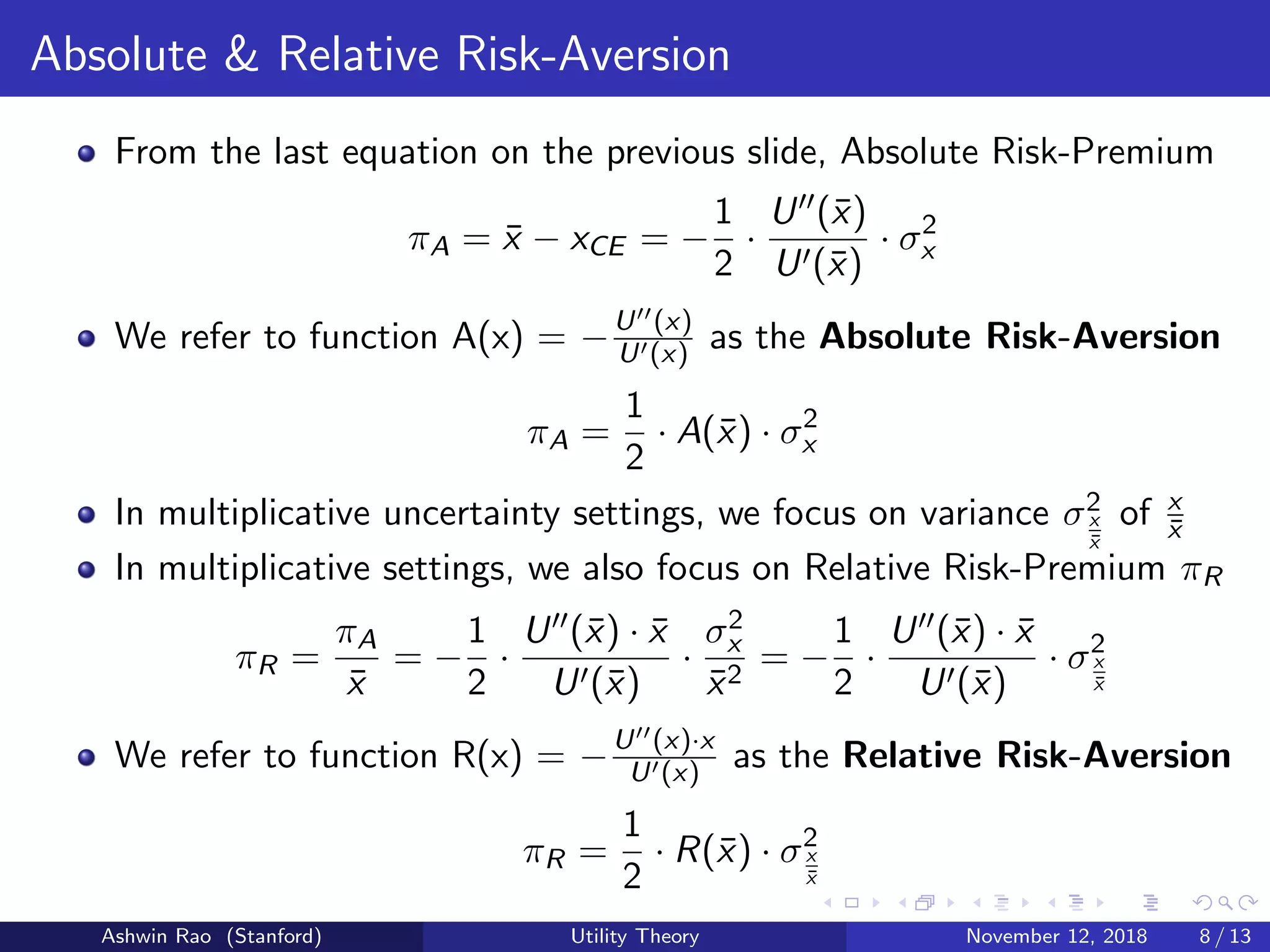
9. Taking stock of what we’re learning here
We’ve shown that Risk-Premium can be expressed as the product of:
Extent of Risk-Aversion: either A(¯x) or R(¯x)
Extent of uncertainty of outcome: either σ2
x or σ2
x
¯x
We’ve expressed the extent of Risk-Aversion as the ratio of:
Concavity of the Utility function (at ¯x): −U (¯x)
Slope of the Utility function (at ¯x): U (¯x)
For optimization problems, we ought to maximize E[U(x)] (not E[x])
Linear Utility function U(x) = a + b · x implies Risk-Neutrality
Now we look at typically-used Utility functions U(·) with:
Constant Absolute Risk-Aversion (CARA)
Constant Relative Risk-Aversion (CRRA)
Ashwin Rao (Stanford) Utility Theory November 12, 2018 9 / 13

10. Constant Absolute Risk-Aversion (CARA)
Consider the Utility function U(x) = −e−ax
Absolute Risk-Aversion A(x) = −U (x)
U (x) = a
a is called Coefficient of Constant Absolute Risk-Aversion (CARA)
If the random outcome x ∼ N(µ, σ2),
E[U(x)] = −e−aµ+a2σ2
2
xCE = µ −
aσ2
2
Absolute Risk Premium πA = µ − xCE =
aσ2
2
For optimization problems where σ2 is a function of µ, we seek the
distribution that maximizes µ − aσ2
2
Ashwin Rao (Stanford) Utility Theory November 12, 2018 10 / 13

11. Constant Relative Risk-Aversion (CRRA)
Consider the Utility function U(x) = x1−γ
1−γ for γ = 1
Relative Risk-Aversion R(x) = −U (x)·x
U (x) = γ
γ is called Coefficient of Constant Relative Risk-Aversion (CRRA)
For γ = 1, U(x) = log(x) (note: R(x) = −U (x)·x
U (x) = 1)
If the random outcome x is lognormal, with log(x) ∼ N(µ, σ2),
E[U(x)] =



eµ(1−γ)+ σ2
2 (1−γ)2
1−γ for γ = 1
µ for γ = 1
xCE = eµ+σ2
2
(1−γ)
Relative Risk Premium πR = 1 −
xCE
¯x
= 1 − e−σ2γ
2
Ashwin Rao (Stanford) Utility Theory November 12, 2018 11 / 13

12. A Portfolio application of CRRA (Merton 1969)
We work in the setting of Merton’s 1969 Portfolio problem
We only consider the single-period (static) problem with 1 risky asset
Riskless asset: dRt = r · Rt · dt
Risky asset: dSt = µ · St · dt + σ · St · dzt (i.e. Geometric Brownian)
We are given wealth W0 at time 0, and horizon is denoted by time T
Determine constant fraction π of Wt to allocate to risky asset
To maximize Expected Utility of wealth WT at time T
Note: Portfolio is continuously rebalanced to maintain fraction π
So, the process for wealth Wt is given by:
dWt = (r + π · (µ − r)) · Wt · dt + π · σ · Wt · dzt
Assume CRRA, i.e. Utility function is U(WT ) =
W 1−γ
T
1−γ , 0 < γ = 1
Ashwin Rao (Stanford) Utility Theory November 12, 2018 12 / 13

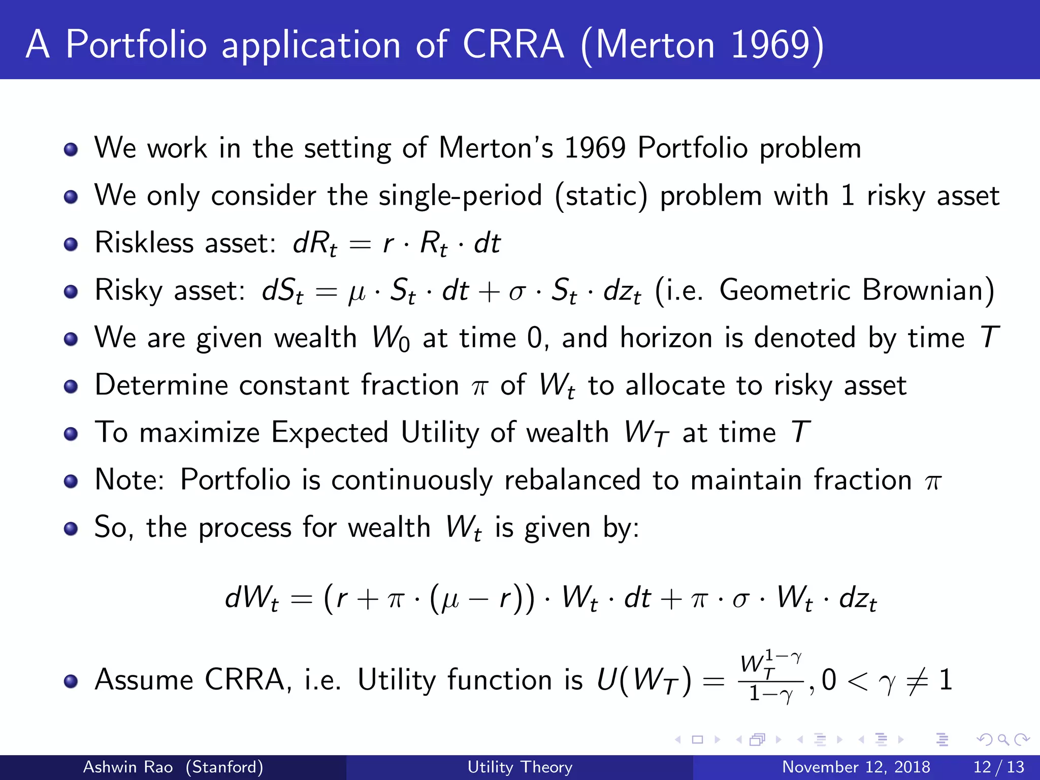
13. Recovering Merton’s solution (for this static case)
Applying Ito’s Lemma on log(Wt) gives us:
WT = W0 · e
T
0 (r+π(µ−r)−π2σ2
2
)·dt+ T
0 π·σ·dzt
We want to maximize log(E[U(WT )]) = log(E[
W 1−γ
T
1−γ ])
E[
W 1−γ
T
1 − γ
] =
W 1−γ
0
1 − γ
· E[e
T
0 (r+π(µ−r)−π2σ2
2
)·(1−γ)·dt+ T
0 π·σ·(1−γ)·dzt
]
=
W 1−γ
0
1 − γ
· e(r+π(µ−r)−π2σ2
2
)(1−γ)T+
π2σ2(1−γ)2T
2
∂{log(E[
W 1−γ
T
1−γ ])}
∂π
= (1 − γ) · T ·
∂{r + π(µ − r) − π2σ2γ
2 }
∂π
= 0
⇒ π =
µ − r
σ2γ
Ashwin Rao (Stanford) Utility Theory November 12, 2018 13 / 13