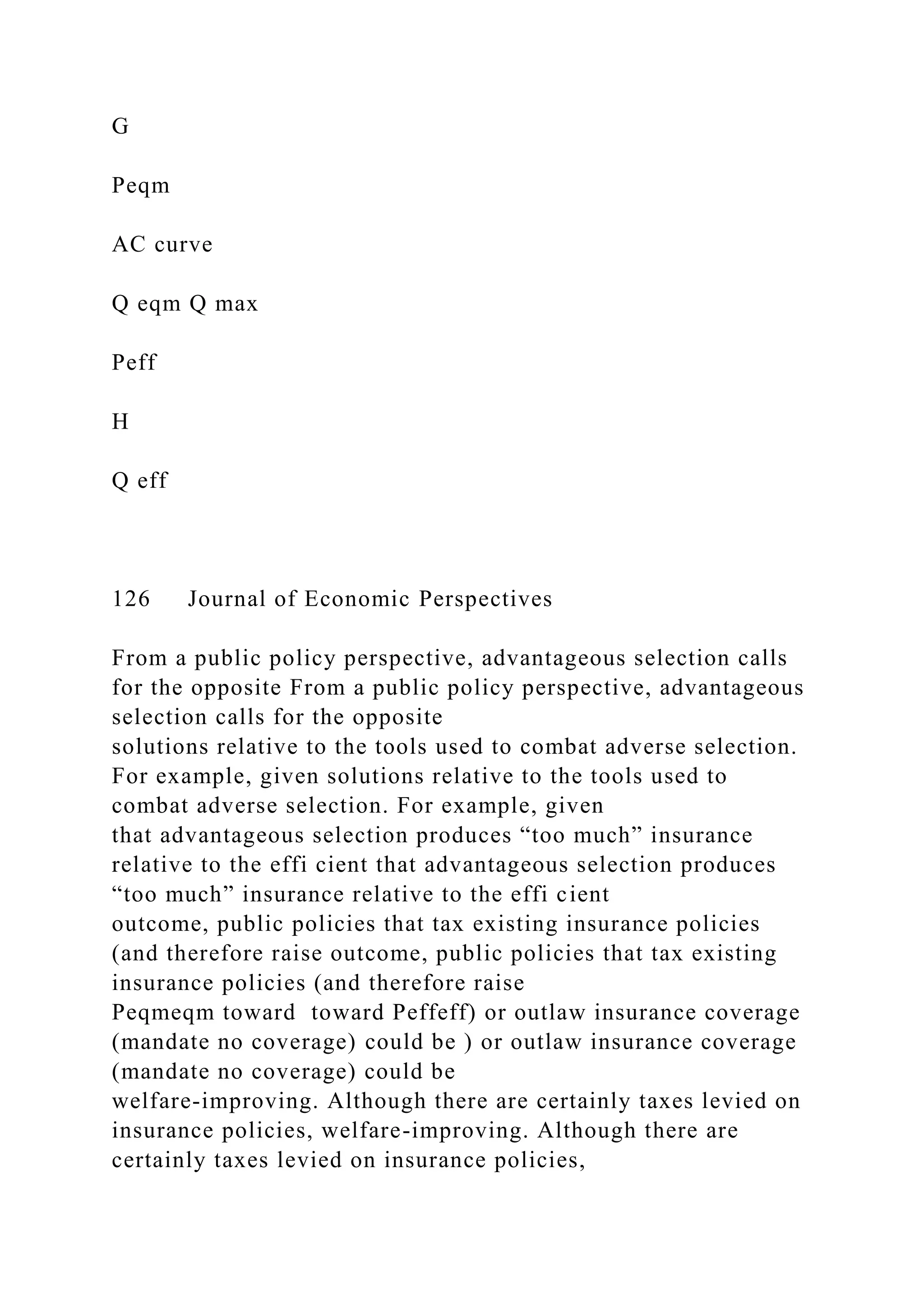
ECON 417 Economics of UncertaintyContentsI Expected U.docx

ECON 417: Economics of Uncertainty
Contents
I Expected Utility Theory 3
1 Lotteries 3
2 St. Petersburg’s Paradox 3
3 von Neumann and Morgenstern Axioms and Expected Utility
Form 4
4 Risk Attitudes 5
5 Risk Premium and Certainty Equivalent 6
6 Measures of Risk Aversion 6
II Mean-Variance Optimization 8
7 One Riskfree Asset, One Risky Asset 8
8 Many Risky Assets 9
9 One Riskfree Asset, Many Risky Assets 9
10 Diversification 10
11 Capital Asset Pricing Model 10
III Insurance 11

12 Utility Maximization 11
12.1 Tangency Condition . . . . . . . . . . . . . . . . . . . . . . . . . . . .
. . . . . . . . . 11
12.2 Substitution Method . . . . . . . . . . . . . . . . . . . . . . . . . . . .
. . . . . . . . . 12
12.3 Lagrange Multipliers . . . . . . . . . . . . . . . . . . . . . . . . . . . .
. . . . . . . . . 12
1
13 State Preference Approach to Insurance 13
14 Overview of Insurance 15
15 Demand for Insurance 15
15.1 Mossin’s Theorem . . . . . . . . . . . . . . . . . . . . . . . . . . . . . .
. . . . . . . . . 16
15.1.1 Actuarially Fair . . . . . . . . . . . . . . . . . . . . . . . . . . . . . .
. . . . . . 16
15.1.2 Not Actuarially Fair . . . . . . . . . . . . . . . . . . . . . . . . . . .
. . . . . . . 16
15.2 Comparative Statics . . . . . . . . . . . . . . . . . . . . . . . . . . . . .
. . . . . . . . 17
15.3 Coinsurance and Deductibles . . . . . . . . . . . . . . . . . . . . . .
. . . . . . . . . . 17

16 Supply of Insurance 18
16.1 Risk pooling . . . . . . . . . . . . . . . . . . . . . . . . . . . . . . . . . .
. . . . . . . . 18
16.2 Risk spreading . . . . . . . . . . . . . . . . . . . . . . . . . . . . . . . .
. . . . . . . . . 19
16.3 “Undersupply” of Full Insurance . . . . . . . . . . . . . . . . . . .
. . . . . . . . . . . 19
17 Asymmetric Information 20
17.1 Adverse Selection . . . . . . . . . . . . . . . . . . . . . . . . . . . . . .
. . . . . . . . . 20
17.1.1 Basic model . . . . . . . . . . . . . . . . . . . . . . . . . . . . . . . . .
. . . . . 20
17.1.2 Tangency Condition . . . . . . . . . . . . . . . . . . . . . . . . . . .
. . . . . . 21
17.1.3 Two types of consumers, symmetric information . . . . . .
. . . . . . . . . . 22
17.1.4 Two types of consumers, asymmetric information . . . . . .
. . . . . . . . . 23
17.1.5 Pooling Equilibrium . . . . . . . . . . . . . . . . . . . . . . . . . . .
. . . . . . 24
17.1.6 Separating Equilibrium . . . . . . . . . . . . . . . . . . . . . . . . .
. . . . . . 25
17.2 Moral Hazard . . . . . . . . . . . . . . . . . . . . . . . . . . . . . . . . .

. . . . . . . . 26
IV After the Midterm 27
17.3 Insurance (cont.) . . . . . . . . . . . . . . . . . . . . . . . . . . . . . . .
. . . . . . . . 27
18 The Value of Information 27
19 Options 27
19.1 Financial Options . . . . . . . . . . . . . . . . . . . . . . . . . . . . . .
. . . . . . . . . 27
19.2 Real Options . . . . . . . . . . . . . . . . . . . . . . . . . . . . . . . . . .
. . . . . . . . 27
2
Part I
Expected Utility Theory
1 Lotteries
For decision making under uncertainty, we consider lotteries.
Lotteries are representations of risky alternatives.
Definition 1 (Simple Lottery). A simple lottery L is a list L =
(p1, ..., p N ) with pi ≥ 0 for all N and∑N
i =1 pi = 1, where pi is the probability of outcome i occurring.
The outcomes that may result

are certain: x1, ..., xN .
Definition 2 (Compound Lottery). A compound lottery is a
lottery in which the outcomes are
simple lotteries.
We can find the probability of each outcome (terminal node) in
a compound lottery by multi-
plying the probabilities of the branches leading to the outcome.
Definition 3 (Reduced Lottery). The overall probability measure
R on X is a simple lottery that
we call the reduced lottery of the compound lottery.
R = x1P (x1) + ... + xN P (xN )
The theoretical analysis of expected utility rests on the
consequentialist premise:
We assume that for any risky alternative, only the reduced
lottery over final outcomes is of rel-
evance to the decision maker.
2 St. Petersburg’s Paradox
Suppose someone offers to toss a fair coin repeatedly until it
comes up heads, and
to pay you $1 if this happens on the first toss, $2 if it takes two
tosses to land a head,
$4 if it takes three tosses, $8 if it takes four tosses, etc.
Question: How much is the lottery worth? How much are you
willing to pay to play this lottery?

3
Expected value of the St. Petersburg problem:
E (X ) =
∞∑
i =1
pi xi
= ( 1
2
) · 1 + ( 1
2
)2 · 2 + ( 1
2
)3 · 4 + ...
= ∞
Paradox: If I charged $1 million to play the game, I would
surely have no takers, despite the fact
that $1 million is still considerably less than the expected value
of the game.
Bernoulli:
• argued that individuals do not care directly about the dollar
prizes of a game; rather they

care about the utility of prizes
• considered u(x ) = log x , which exhibits diminishing marginal
utility
3 von Neumann and Morgenstern Axioms and Expected Utility
Form
von Neumann and Morgenstern describe necessary and
sufficient conditions for the represen-
tation of a utility function.
In expected utility theory, preference relations, %, are
characterized by 3 axioms:
1. Weak-Order requires that the preference relation be complete
and transitive
• Completeness requires that all elements are comparable.
For L1, L2 ∈ L , the preference relation is complete if either L1
% L2 or L2 % L1
• Transitivity requires that choices be consistent.
For L1, L2, L3 ∈ L , the preference relation is transitive if L1
% L2 and L2 % L3 implies
L1 % L3
2. Continuity means that small changes in probabilities do not
change the nature of the
ordering between two lotteries
If L1, L2 ∈ L are such that L1 % L2, then for all L3 ∈ L ,
there is an α such that 0 < α < 1 and L1 Â (1 −α)L2 +αL3
and there is a β such that 0 < β < 1 and (1 −β)L1 +βL3 Â L2

4
For example, if a “beautiful and uneventful trip by car” is
preferred to “staying home,”
then a mixture of the outcome “beautiful and uneventful trip by
car” with a sufficiently
small but positive probability of “death by car accident” is still
preferred to “staying home.”
3. Independence (of irrelevant alternatives) means that if we
mix each of the two lotteries
with a third one, then the preference ordering of the two
resulting mixtures is indepen-
dent of the particular third lottery used
For all lotteries L1, L2, L3 ∈ L and all α such that 0 < α < 1,
L1 Â L2 ⇐⇒ αL1 + (1 −α)L3 % αL2 + (1 −α)L3
The Allais Paradox is a violation of the Independence Axiom.
Theorem 1 (Expected Utility Theorem). If the decision maker’s
preferences over lotteries satisfy
the weak-order, continuity, and independence axioms, then her
preferences are representable by
a utility function with the expected utility form.
EU (L) =
N∑
i =1

pi u(xi ) = p1u(x1) + ... + p N u(xN )
Criteria for Maximization
L1 % L2 ⇐⇒ EU (L1) ≥ EU (L2)
4 Risk Attitudes
Risk aversion captures the idea that individuals dislike risk and
uncertainty.
Definition 4 (Fair bet). A fair bet is a random game with a
specified set of prizes and associated
probabilities that has an expected value of zero.
Definition 5 (Concavity). The function f (x ) is concave if a
straight line joining any two points
on it lies entirely below the function itself. In other words, the
function f (x ) is concave if for
any x1 and x2, and λ : 0 ≤ λ ≤ 1,
f (λx1 + (1 −λ)x2) ≥ λf (x1) + (1 −λ) f (x2)
If f (x ) is a concave (twice differentiable) function, then f ′′(x )
< 0.
A decision maker is risk averse if
5
1. at any level of wealth, he rejects every fair bet
2. he strictly prefers a certainty consequence to any risky

prospect whose mathematical ex-
pectation of consequences equals that certainty
3. u(x ) is concave. In other words, for every lottery with
outcomes x1, ..., xN and probabili-
ties p1, ..., p N , respectively
u(
N∑
i =1
pi xi ) ≥
N∑
i =1
pi u(xi )
Concavity of the utility function implies diminishing marginal
utility.
A decision maker is risk loving if
1. at any level of wealth, he accepts every fair bet
2. he strictly prefers the lottery to its mathematical expectation
3. u(x ) is convex. In other words, for every lottery with
outcomes x1, ..., xN and probabilities
p1, ..., p N , respectively
u(
N∑

i =1
pi xi ) ≤
N∑
i =1
pi u(xi )
A decision maker is risk neutral if
1. at any level of wealth, he is indifferent to every fair bet
2. he is indifferent between the lottery and its mathematical
expectation
5 Risk Premium and Certainty Equivalent
Definition 6 (Certainty Equivalent). The amount of money, C E
(L), when obtained for certain,
provides the same expected utility as the lottery
Definition 7 (Risk Premium). The maximum amount, π, that an
individual is willing to forego
in order to receive the expected value of the lottery with
certainty
The risk premium is the difference between the expected value
of the lottery and the certainty
equivalent of the lottery.
π = E (L) −C E (L)
6 Measures of Risk Aversion

The Arrow-Pratt measures of risk aversion are quantitative
measures of how averse to risk a
person is. It provides a way to measure the degree of concavity
of the utility function (hence,
the strength or intensity of risk aversion).
6
Definition 8 (Absolute Risk Aversion). The absolute risk
aversion measure A(x ) for a utility
function u(x ) is
A(x ) ≡ −u
′′(x )
u(x )
Definition 9 (Relative Risk Aversion). The relative risk
aversion measure R (x ) for a utility func-
tion u(x ) is
R (x ) ≡ −x u
′′(x )
u(x )
= x · A(x )
Definition 10 (DARA, CARA, IARA). The utility function u(·)
has decreasing (constant, increas-
ing) absolute risk aversion if A(x , u) is a decreasing (constant,
increasing) function of x . This

depends on the sign of the derivative of A(x ) with respect to x ,
i.e. d A(x )d x .
Empirical evidence supports DARA. The power utility function
exhibits DARA.
Definition 11 (DRRA, CRRA, IRRA). The utility function u(·)
has decreasing (constant, increas-
ing) relative risk aversion if R (x , u) is a decreasing (constant,
increasing) function of x . This
depends on the sign of the derivative of R (x ) with respect to x
, i.e. d R (x )d x .
7
Part II
Mean-Variance Optimization
V (µ,σ)
• µ is the expected return of the asset
• σ is the standard deviation of the asset. Risk is measured by
the standard deviation.
Risk attitudes are determined by the partial derivatives with
respect to risk
• δV
δσ
< 0 risk averse

• δV
δσ
> 0 risk loving
• δV
δσ
= 0 risk neutral
Typically, financial economists think of investors as being risk
averse, thus investors trade off
risk and return.
The risk-return tradeoff:
• A risk averse, mean-variance optimizing investor will only
accept a riskier portfolio if the
expected return of that portfolio is appropriately higher
• A risk averse, mean-variance optimizing investor will only
accept a portfolio that has a
lower expected return if the risk of that portfolio is
appropriately lower
Consider the particular functional form for a mean-variance
optimizer:
V (µ,σ) = µ− 1
2
A ·σ2
where µ is expected return, σ2 is the variance, and A is the

coefficient of risk aversion ( A > 0).
7 One Riskfree Asset, One Risky Asset
Assume that an investor must decide how to invest all of her
wealth and has only two options:
a riskfree asset, R f and a risky asset. The expected return of the
risky asset is E (Ri ) and its
variance is V ar (Ri ) = σ2i . To determine the optimal fraction
of wealth an investor will allocate
to a risky asset, k∗ , consider the following maximization
problem
max
k
V (µp ,σp ) = µp −
1
2
A ·σ2p
= E (Rp ) −
1
2
A · V ar (Rp )
= R f + k (E (Ri ) − R f ) −
1
2
A · k 2V ar (Ri )

8
Solve the optimization problem. The first-order condition
requires that the derivative, with
respect to k , is equal to zero. We find
k∗ =
(E (Ri ) − R f )
A · V ar (Ri )
= S
A ·σi
Definition 12 (Sharpe Ratio). The Sharpe Ratio, S of the risky
asset is the expected excess re-
turn of the risky asset per unit of its standard deviation. It is the
reward-to-variability ratio of
investing in the risky asset.
S =
E (Ri ) − R f
σi
Definition 13 (Capital Allocation Line). A graph of all possible
expected returns and standard
deviations of a portfolio formed by combining the risky asset
with the riskfree asset.
8 Many Risky Assets
Consider a portfolio of two assets with weights k1 and k2,

expected returns E (R1) and E (R2),
and return variances σ21 and σ
2
2.
The portfolio expected return is
E (Rp ) = k1E (R1) + k2E (R2)
The portfolio variance is
V ar (RP ) = k 21σ21 + k 22σ22 + 2 · k1 · k2 ·C ov (R1, R2)
The graph is a hyperbola when volatility is plotted on the x-axis
and expected returns are plotted
on the y-axis.
Definition 14 (Efficient Frontier). A graph of the feasible
investments with the highest expected
returns for all possible portfolio standard deviations. It is the
top part of the graph above the
minimum variance portfolio.
9 One Riskfree Asset, Many Risky Assets
Definition 15 (Capital Market Line). The line from the riskfree
investment through the efficient
portfolio of risky assets when volatility is plotted on the x-axis
and expected returns are plotted
on the y-axis.
9

Definition 16 (Tangency Portfolio). The portfolio of risky assets
with the highest Sharpe Ratio.
It is an efficient portfolio and it generates the steepest line
combined with the riskfree asset.
Theorem 2 (Mutual Fund (Separation) Theorem). Investors with
the same beliefs about expected
returns, risks, and correlations all will invest in the portfolio or
“fund” of risky assets that has the
highest Sharpe Ratio, but they will differ in their allocations
between this fund and the riskfree
asset based on their risk tolerance.
10 Diversification
The risk of a stock includes idiosyncratic risk and market risk.
Idiosyncratic risk is also known
as firm-specific, unique, stand-alone, or diversifiable risk.
Market risk is also known as system-
atic or undiversifiable risk.
To limit your exposure to idiosyncratic risk, you can diversify
your portfolio. This means choos-
ing stocks that are imperfectly correlated, i.e. ρ → −1, where ρ
is the correlation coefficient.
The benefit of diversification will increase the further away
from ρ = 1.
Definition 17 (Risk premium). It represents the additional return
that investors expect to earn
to compensate them for a security’s risk. It is the difference

between the expected return of the
security minus the riskfree rate of return.
E (Ri ) − R f
11 Capital Asset Pricing Model
Intuition for the Capital Asset Pricing Model (CAPM)
1. Because diversification does not reduce market risk, the risk
premium of a security should
be determined by its market risk.
2. To measure market risk, we need a market portfolio. If all
investors are mean-variance
optimizers, by the Mutual Fund Theorem, they should be
holding the Tangent Portfolio.
Let the Market Portfolio be the Tangent Portfolio.
CAPM relates the security’s risk premium to the market risk
premium.
E (Ri ) − R f = β· (E (Rm ) − R f )
and β, which measures the sensitivity of the security’s return to
the return of the overall market
is
β = C ov (Ri , Rm )
V ar (Rm )

10
Part III
Insurance
12 Utility Maximization
There are three methods you can use to solve the utility
maximization problem:
max
x1 ,x2
u(x1, x2) subject to their budget constraint: I = p1 x1 + p2 x2
12.1 Tangency Condition
The slope of the indifference curve and the slope of the budget
line should be equal at the point
of tangency. It is the point at which the consumer maximizes his
or her utility, given his or her
budget constraint.
slope of indifference curve = slope of budget line
MRSx1 x2 =
p1
p2
MU1
MU2

= MRSx1 x2 =
p1
p2
Example 1. Suppose we had the following utility function
max
x1 ,x2
u(x1, x2) = log x1 + log x2 subject to their budget constraint: I
= p1 x1 + p2 x2
1
x1
1
x2
= p1
p2
⇒ x2 =
p1
p2
x1
Plug into the budget constraint
I = p1 x1 + p2 x2
I = p1 x1 + p2
p1

p2
x1
I = 2p1 x1
⇒ x∗ 1 =
I
2p1
and x∗ 2 =
I
2p2
11
12.2 Substitution Method
Example 2. Consider the following constrained problem with
two variables
max
x1 ,x2
log x1 + log x2
s.t
p1 x1 + p2 x2 = I
The idea of the substitution method is to use the constraints to
get rid of some variables. In the

example above we can use the constraint to obtain that x2 = I
−p1 x1p2 , and after we plug this into
the objective function we get
ũ(x1) = log x1 + log
I − p1 x1
p2
This becomes an unconstrained maximization problem for a
function of one variable x1. Using
the chain rule we obtain the following first order condition
(FOC)
0 = ũ′(x1) =
1
x1
+ p2
I − p1 x1
(−p1
p2
)
= 1
x1
− p1
I − p1 x1
which yields I − p1 x1 = p1 x1, the solution of this equation is
x∗ 1 = I2p1 .
By the chain rule and the power rule we have

ũ′′(c1) = −
1
x 21
− (−1)(−p1)
p1
(I − p1 x1)2
= − 1
x 21
−
p 21
(I − p1 x1)2
Clearly ũ′′(c1) < 0 for any x1 and so the sufficient condition for
a local maximum is satisfied.
Finally, using the constraint p1 x
∗
1 + p2 x∗ 2 = I we get x∗ 2 = I2p2 , so the solution of the
problem is
the consumption bundle (x∗ 1 , x
∗
2 ) = ( I2p1 ,
I
2p2
).
12.3 Lagrange Multipliers

Theorem 3. Let f and g be two real-valued continuously
differentiable functions of two vari-
ables. Suppose that (x∗ 1 , x
∗
2 ) is a solution to the following maximization problem
max
x1 ,x2
f (x1, x2)
subject to
g (x1, x2) = 0
and that (x∗ 1 , x
∗
2 ) is not a critical point of g . Then there exists a real number λ
∗ called the lagrange
multiplier, such that (x∗ 1 , x
∗
2 ,λ
∗ ) is a critical point of the following function, called a
Lagrangian
L (x1, x2,λ) = f (x1, x2) +λg (x1, x2)
12
i.e. all three partial derivatives of L are zero

∂L
∂x1
(x∗ 1 , x
∗
2 ,λ
∗ ) = 0
∂L
∂x2
(x∗ 1 , x
∗
2 ,λ
∗ ) = 0
∂L
∂λ
(x∗ 1 , x
∗
2 ,λ
∗ ) = 0
Example 3. Let’s apply the Lagrange Theorem to the
consumer’s problem from previous sec-
tion.
max
x1 ,x2

log x1 + log x2
s.t. p1 x1 + p2 x2 = I
The objective function is f (x1, x2) = log x1+log x2, the
constraint function is g (x1, x2) = I −p1 x1−
p2 x2, and the Lagrangian function is
L (x1, x2,λ) = log x1 + log x2 +λ
(
I − p1 x1 − p2 x2
)
From the Lagrange Theorem, the First Order Necessary
Condition is that all partial derivatives
of the Lagrangian are zero, i.e.
∂L
∂x1
(x∗ 1 , x
∗
2 ,λ
∗ ) = 0 ⇒ 1
x∗ 1
−λ∗ p1 = 0
∂L
∂x2
(x∗ 1 , x
∗
2 ,λ

∗ ) = 0 ⇒ 1
x∗ 2
−λ∗ p2 = 0
∂L
∂λ
(x∗ 1 , x
∗
2 ,λ
∗ ) = 0 ⇒ I − p1 x∗ 1 − p2 x∗ 2 = 0
Note that last equation simply says that the constraint in the
maximization problem has to hold.
The above is a system of 3 equations and 3 unknowns (x∗ 1 , x
∗
2 ,λ
∗ ) and is quite easy to solve. We
get:
x∗ 1 =
I
2p1
x∗ 2 =
I
2p2
λ∗ = 2

I
13 State Preference Approach to Insurance
Goal: To show that when faced with fair markets in contingent
claims on wealth, a risk averse
person will choose to ensure that he has the same level of
wealth regardless of which state oc-
curs.
Categorize all of the possible things that might happen into a
fixed number of states. We say
that contingent commodities are goods delivered only if a
particular state of the world occurs.
13
Consider the following expected utility model of two contingent
goods: Wg is wealth in good
times and Wb is wealth in bad times.
max EU (Wg , Wb ) = p u(Wb ) + (1 − p )u(Wg )
Initial wealth is W . Assume that this person can purchase a
dollar of wealth in good times for
qg and a dollar of wealth in bad times for qb .
1 The price ratio
qg
qb

shows how this person can
trade dollars of wealth in good times for dollars in bad times.
W̃ = qb Wb + qg Wg
We say that prices are actuarially fair if the price ratio reflects
the odds ratio:
qg
qb
= 1 − p
p
Example 4. Consider the following expected utility
maximization problem:
max EU (Wg , Wb ) = p log(Wb ) + (1 − p ) log(Wg ) subject to
W̃ = qb Wb + qg Wg
We can use the tangency condition to solve.
1−p
Wg
p
Wb
=
qg
qb
1 − p
p

Wb
Wg
=
qg
qb
Use the condition that insurance is actuarially fair to simplify,
and we get:
Wg = Wb
The individual is willing to pay an indemnity or cover for
reduced wealth in the “good state" so
that he can have the same level of wealth in the event of a loss.
Wg = Wb
W − qC = W − L − qC +C
where L is the loss, C is the cover, qC is the premium expressed
as the the product of the cover
and a premium rate.
1I use q for prices because I don’t want to confuse it with p for
probability.
14
14 Overview of Insurance
Insurance occurs when one party agrees to pay an indemnity (a

promise to pay for the cost of
possible damage, loss, or injury) to another party in case of the
occurrence of a pre-specified
random event generating a loss for the initial risk-bearer.
Definition 18 (Risk transfer). Insurance is the most common
form of risk transfer. The shifting
of risk is of considerable importance for the functioning of our
modern economies.
• Insurance is a particular example of a type of risk-transfer
strategy known as hedging.
Hedging strategies typically involve entering into contracts
whose payoffs are negatively
related to one’s overall wealth or to one component of that
wealth. Thus, for example, if
wealth falls, the value of the contract rises, partially offsetting
the loss in wealth.
The basic characteristics of all insurance contracts are:
• specified loss events
• losses, L
• cover (indemnity), C
• premium, Q . Q = qC is a common, but not universal, way of
expressing the insurance
premium.
15 Demand for Insurance

Question: How much insurance would a risk-averse person buy?
What is the demand for cover?
Answer:
max
C
EU = p u(W − L − qC +C ) + (1 − p )u(W − qC )
The first order condition is:
d EU
d C
= p u′(W − L − qC +C )(1 − q ) − (1 − p )u′(W − qC )q = 0
u′(W − L − qC +C )
u′(W − qC ) =
(1 − p )q
p (1 − q ) > 1
15
15.1 Mossin’s Theorem
15.1.1 Actuarially Fair
We say that insurance is actuarially fair if the expected payout
of the insurance company just
equals the cost of the insurance.
expected payout is probability of loss times the cover =

expected cost is the insurance premium
pC = qC
p = q
We might expect a competitive insurance market to deliver
actuarially fair insurance. In this
case, the first order condition simplifies to:
u′(W − L − qC +C ) = u′(W − qC )
The consumer should fully insure and set the cover equal to the
loss C ∗ = L (full cover).
Mossin’s Theorem states that a risk averse individual offered
insurance at a fair premium will
always choose full cover.
q = p ⇐⇒ u′(W − qC ∗ ) = u′(W − L − qC ∗ +C ∗ ) ⇐⇒ C ∗ = L
15.1.2 Not Actuarially Fair
Question: What happens if the price of insurance is above the
actuarially fair price, i.e. q > p ?
u′(W − L − qC +C )
u′(W − qC ) =
(1 − p )q
p (1 − q ) > 1
Mossin’s Theorem
With a positive loading, the buyer chooses partial cover;
q > p ⇐⇒ u′(W − qC ∗ ) < u′(W − L − qC ∗ +C ∗ ) ⇐⇒ C ∗ < L

With a negative loading the buyer chooses more than full cover;
q < p ⇐⇒ u′(W − qC ∗ ) > u′(W − L − qC ∗ +C ∗ ) ⇐⇒ C ∗ > L
where the last two results follow from the fact that u′(·) is
decreasing in wealth, i.e., from risk
aversion.
16
15.2 Comparative Statics
From the first order condition, we can in principle solve for the
optimal cover as a function of
the exogenous variables of the problem: wealth, the premium
rate, the amount of loss, and the
loss probability. The buyer’s demand for cover function can be
expressed as:
C ∗ = C (L, p, W , Q )
Question: How does the demand for cover change as wealth, the
premium rate (price of insur-
ance), the amount of loss, and the loss probability change?
• Amount of loss, L, i.e. δC
∗
δL . A ceteris paribus increase in L increases the demand for
insur-
ance.

• The loss probability, p , i.e. δC
∗
δp . An increase in the risk of loss increases the demand for
cover.
• Wealth, W , i.e. δC
∗
δW
Proposition 1. If p = q , the agent will insure fully at C ∗ = L
for all wealth levels. If p < q ,
the agent’s insurance coverage as a function of wealth, C ∗ (W )
will decrease (increase)
with wealth if the agent has decreasing (increasing) absolute
risk aversion.
• Premium rate, Q , i.e. δC
∗
δQ . The total effect on insurance demand depends on the
relative
magnitudes of the income and substitution effect.
15.3 Coinsurance and Deductibles
Proposition 2. Under a reasonable set of conditions, the optimal
insurance contract always
takes the form of a straight deductible.
Under proportional coinsurance we have cover

C = αL, α ∈ [0, 1]
with α = 0 implying no insurance and α = 1 implying full cover.
Under a deductible we have
C =
{
0 for L ≤ D
L − D for L > D
where D denotes the deductible and D = 0 implies full cover.
Given the premium amount Q and wealth W in the absence of
loss, the buyer’s state-contingent
wealth in the case of proportional coinsurance is
Wα = W − L −Q +C = W − (1 −α)L −Q
17
and in the case of a deductible is
WD = W − L −Q +C = W − L −Q + max(0, L − D )
For losses above the deductible, her wealth becomes certain,
and equal to
ŴD = W − L −Q + (L − D ) = W −Q − D
A straight deductible insurance policy efficiently concentrates
the effort of indemnification on
only the largest losses.

16 Supply of Insurance
16.1 Risk pooling
When an insurer enters into insurance contracts with a number
of individuals, or a group of
individuals agrees mutually to provide insurance to each other,
the probability distribution of
the aggregate losses they may suffer differs from the loss
distribution facing any one individual.
Assume
• There are i = 1, 2, ..., N individuals with identically and
independently distributed risks
• C̃i is the loss claim for each individual (the cover paid by the
insurance company in the
event of a loss)
• µ is the expected claims cost (across the population) and σ2 is
the variance of the expected
claims costs
• Each C̃i has the same probability distribution with mean µ and
variance σ
2
Let C
̄ N = 1N
∑N
i =1 Ci be the sample mean or average loss per contract (to the

insurance com-
pany).2
Proposition 3 (By the Law of Large Numbers).
lim
N →∞
Pr[|C
̄ N −µ| < ²] = 1
In words, as N becomes increasingly large, the average loss per
contract will be arbitrarily close
to the value µ with probability approaching 1.
2A sample is a (randomly) generated subset of the population
under study. The parameters of the population in-
clude its mean, µ, variance, σ2, and its standard deviation, σ.
The statistics of the sample include the sample mean
(or average), X
̄ = 1N
∑N
i =1 X i , the (unbiased) sample variance is s
2 = 1N −1
∑N
i =1(X i − X
̄ )2, and the sample standard
error is the sample standard deviation divided by the square root
of the sample size, i.e. sp
N
.

18
Stated differently,
for a sufficiently large number of insurance contracts, it is
virtually certain that the loss per
contract is just about equal to the mean of the loss claims
distribution.
Furthermore, the variance of the realized loss per contract about
the mean of loss claims goes
to zero as N becomes increasingly large.
Var(C
̄ N ) = Var(
1
N
N∑
i =1
Ci ) =
1
N 2
· Nσ2 = σ
2
N
16.2 Risk spreading

When risks are not covered by insurance companies, the
government can intercede by transfer-
ring money among parties. The government can spread the risk
to increase social welfare.
As a risk is spread over an increasing number of individuals, the
total cost of the risk tends to
zero and the price individuals are willing to pay for the risky
prospect tends to the expected
value of the project.
Theorem 4 (Arrow-Lind). Under certain assumptions, the social
cost of risk moves to zero as
the population tends to infinity, so that projects can be
evaluated on the basis of expected net
benefit alone. A necessary condition for the results is that the
covariance between the individual’s
wealth from the insurance business and his marginal utility of
wealth, if he does not share in this
business, must be zero.
The Arrow-Lind Theorem provides a basis for the assumption
that the insurer is risk neutral.
16.3 “Undersupply” of Full Insurance
1. Transactions (or insurance) costs include: drawing up and
selling new insurance con-

tracts, administering the stock of existing contracts, processing
claims, estimating loss
probabilities, calculating premiums, and administering the
overall business. The Raviv
model shows how the existence of deductibles and coinsurance
in the (equilibrium) in-
surance contract is related to the nature of insurance costs.
2. Nondiversifiable risks cannot be insured.
3. Adverse selection: individuals know their risk better than the
insurance company
4. Moral hazard: individuals can take certain actions to reduce
the probability of loss
19
17 Asymmetric Information
Markets may not be fully efficient when one side has
information that the other side does not
(asymmetric information). Carefully designed contracts may
reduce such problems by provid-
ing incentives to reveal one’s information and take appropriate
actions.
Principal-Agent Model
There are two economic agents in this model: the informed

party and the uninformed party.
One party will propose a “take it or leave it” (TIOLI) contract
and therefore request a “yes or no”
answer; the other party is not free to propose another contract.
The principal is the one who
proposes the contract and the agent is the party who just has to
accept or reject the contract.
Hidden Type
The uninformed party is imperfectly informed of the
characteristics of the informed party; the
uninformed party moves first. The agent has private information
about the state of the world
before signing the contract with the principal. The agent’s
private information is called his type.
For historical reasons stemming from its application in the
insurance context, the hidden-type
model is also called an adverse selection model.
Hidden Action
The uninformed party moves first and is imperfectly informed
of the actions of the informed
party. The agent’s actions taken during the term of the contract
affect the principal, but the
principal does not observe these actions directly. The principal
may observe outcomes that

are correlated with the agent’s actions but not the actions
themselves. For historical reasons
stemming from the insurance context, the hidden-action model
is called a moral hazard model.
17.1 Adverse Selection
Adverse selection is defined as the situation where the insured
has better information about
her risk type than the insurer. We then say that the individual
risk is her private information.
We will consider the Rothschild and Stiglitz (1976) model of
adverse selection in competitive
insurance markets.
17.1.1 Basic model
Basic Model
• The individual is risk averse
• Individual is endowed with wealth, W
• In the event of a loss, the individual will have W − L
• p is the probability of the loss
20
• He can insure himself by paying a premium Q = qC in return
for a cover C , if a loss occurs

• The pair (Q , C ) completely describes the insurance contract
• Insurance contracts are exclusive: each individual can take on
only a single insurance
contract
Demand for Insurance
EU = p u(Wb ) + (1 − p )u(Wg )
where u(x ) is the utility of money income; u(x) is an increasing
concave function. An individual
chooses the insurance contract that maximizes his expected
utility.
Supply of Insurance
• Companies are risk neutral and are concerned only about
expected profits:
π = Q − pC
• A perfectly competitive market ⇒ zero economic profits
• Zero administrative costs
• Free entry
• Each firm can offer only one contract
Equilibrium in a competitive insurance market is a set of
contracts such that when individuals
choose contracts to maximize expected utility
1. No contract in the equilibrium set makes negative expected
profits

2. No contract outside the equilibrium set that, if offered, will
make a nonnegative profit
Every firm makes zero profits and no firm (existing or new) can
make positive profits by offering
a new contract.
17.1.2 Tangency Condition
Budget Line
Final wealth in the two states of the world are
W̃ =
{
Wg = W − qC in “good” state
Wb = W − L + (1 − q )C in “bad” state
To find the budget line, multiply Wg by (1 − q ) and Wb by (q ).
Then add the two equations.
(1 − q )Wg + qWb = W − qC − qW + q 2C + qW − q L + qC − q
2C
= (1 − q )W + q (W − L)
= W − q L
21
Solve for Wb and you’ll get
Wb =
W − q L

q
− 1 − q
q
Wg
This is a straight line passing through the point (W , WL ), i.e.
the no insurance point, and having
a negative slope equal to
1−q
q in absolute value.
Marginal Rate of Substitution (MRS)
Recall from microeconomics that the marginal rate of
substitution is the slope of the indiffer-
ence curve, i.e. M R S = − x1x2 . It describes how much x2 a
person is willing to give up in order
to get more x1 and remain indifferent between the two
consumption bundles. For example, if
M R S = 5 then the consumer is willing to give up 5 units of x2
to get one unit of x1. The M R S is
also equal to the ratio of the marginal utilities.
From the expected utility maximization function, we find that
M R S =
MUW g
MUW b
= (1 − p )
p

u′(Wg )
u′(Wb )
17.1.3 Two types of consumers, symmetric information
Suppose that the market consists of two kinds of customers:
• low risk individuals with loss probability, pL
• high risk individuals with loss probability, p H
• Note that 1 > p H > pL > 0
22
The MRS for each type is
M R SL =
(1 − pL )
pL
u′(Wg )
u′(Wb )
andM R S H =
(1 − p H )
p H
u′(Wg )
u′(Wb )
The slope of the indifference curve of low risks is steeper than
that of high risks.

In the first-best, symmetric information case, the insurance
company can observe the individ-
ual’s risk type and offer a different policy to each. In the
competitive market, each type can get
a separate contract with an actuarially fair premium and chooses
full coverage.
17.1.4 Two types of consumers, asymmetric information
Question: What happens when the individual has private (not
observable or verifiable) infor-
mation about his type?
Intuition: If the same full insurance contracts for each group
were offered, but types are not
observable, then all individuals would choose the low type
insurance contract. This could lead
to negative profits for the firm. Why? Insurers break even
serving only the low-risk types, so
adding individuals with a higher probability of loss would push
the company below the break-
even point. Therefore, we cannot offer full insurance to both
types.
23
There are two types of equilibria to consider: pooling and
separating.

Definition 19 (Pooling equilibrium). Pooling equilibrium in a
competitive screening model is
an equilibrium where each type of agent chooses the same
contract.
Definition 20 (Separating equilibrium). A separating
equilibrium is a competitive screening
model is where different types purchase different contracts.
17.1.5 Pooling Equilibrium
Proposition 4. There cannot be a pooling equilibrium.
Intuition: The pooling equilibrium cannot be a final equilibrium
because there exist insurance
policies that are unattractive to high-risk types, attractive to
low-risk types, and profitable to in-
surers. These policies will involve “cream-skimming” behavior:
the policies will attract low-risk
types away from the pooling contract. The insurers that
continue to offer the pooling contract
are left with individuals whose risk is so high that insurers
cannot expect to earn any profit by
serving them.
24
17.1.6 Separating Equilibrium

Proposition 5. The separating equilibrium will involve
actuarially fair full insurance for the
high risk types and low risk individuals will be offered the best
possible partial insurance con-
tract at a fair price, conditional on that contract being
unattractive to high-risk individuals.
Definition 21 (Incentive compatibility constraints). The
incentive compatibility (IC) constraints
state that each consumer prefers the contract that was designed
for him.
Intuition: We need to consider incentive compatibility
constraints. There is no reason to distort
the choice of insurance for the high-risk types, because low risk
individuals do not have any
incentive to “pretend” to be high risk. But we need to make sure
the high risk types don’t pretend
to be low risk types. The incentive compatibility constraint for
the high type requires that the
contract designed for the low risk type be below or on the
indifference curve of the high risk
type that goes through the full insurance contract.
25
Existence of a separating equilibrium:
“An equilibrium will not exist if the costs to the low-risk
individual of pooling are low (because

there are relatively few of the high-risk individuals who have to
be subsidized, or because the
subsidy per individual is low, i.e. when the probabilities of the
two groups are not too different),
or if their costs of separating are high” (Rothschild and Stiglitz,
1976).
17.2 Moral Hazard
In the moral hazard model of insurance, the probability of the
loss state may depend on the
behavior of the insured individual. This creates an incentive
problem that leads to less than full
insurance, so that the insured retains some incentive to behave
differently.
Suppose
• a risk-averse individual faces the possibility of incurring a
loss, L, that will reduce his
wealth, W
• the probability of loss is p and is a decreasing convex function
of effort, e (or level of care)
• exerting effort is costly, i.e. c (e ) in an increasing function in
effort; let c (e ) = e (The insur-
ance company cannot monitor the individual’s level of effort, e
).

• u(x ) is the individual’s utility given wealth
The individual’s expected utility as a function of the effort or
level of care chosen is
EU = p (e )u(Wb ) + (1 − p (e ))u(Wg )
= p (e )u(W − e −Q − L +C ) + (1 − p (e ))u(W − e −Q )
26
The expected profit of the (risk-neutral) insurance company is
π = Q − p (e )C
An actuarially fair insurance contract would set a premium
equal to the expected coverage, i.e.
Q = p (e )C .
The timing is as follows:
• The principal offers an insurance contract (Q , C )
• The individual decides to accept or reject the contract
• The individual chooses an effort level, e
Definition 22 (Participation Constraint). The participation, or
individually rational (IR), con-
straint guarantees that the consumer will accept the contract.
The individual must be at least
as well off as he would be if he accepted the next best
alternative. (No insurance may be the

next best alternative).
In our setting, the optimal contract must
• satisfy the zero-profit constraint (the IR constraint for the
firm)
• satisfy the IR or participation constraint for the individual
• ensure that the effort level in the contract is credible in the
sense that it will be chosen by
the agent under the incentives provided by the rest of the
contract.
Part IV
After the Midterm
17.3 Insurance (cont.)
18 The Value of Information
19 Options
19.1 Financial Options
19.2 Real Options
27
Journal of Economic Perspectives—Volume 25, Number 1—
Winter 2011—Pages 115–138

FF rom the large-scale social insurance programs of Social
Security and Medi-rom the large-scale social insurance
programs of Social Security and Medi-care to the heavily
regulated private markets for property and casualty care to the
heavily regulated private markets for property and casualty
insurance, government intervention in insurance markets is
ubiquitous. The insurance, government intervention in insurance
markets is ubiquitous. The
fundamental theoretical reason for such intervention, based on
classic work from fundamental theoretical reason for such
intervention, based on classic work from
the 1970s, is the problem of adverse selection. But despite the
age and infl uence the 1970s, is the problem of adverse
selection. But despite the age and infl uence
of the theory, systematic empirical examination of selection in
actual insurance of the theory, systematic empirical examination
of selection in actual insurance
markets is a relatively recent development. Indeed, in awarding
the 2001 Nobel markets is a relatively recent development.
Indeed, in awarding the 2001 Nobel
Prize for the pioneering theoretical work on asymmetric
information to George Prize for the pioneering theoretical work
on asymmetric information to George
Akerlof, Michael Spence, and Joseph Stiglitz, the Nobel
committee noted this Akerlof, Michael Spence, and Joseph
Stiglitz, the Nobel committee noted this
paucity of empirical work (Nobelprize.org, 2001).paucity of
empirical work (Nobelprize.org, 2001).
Over the last decade, however, empirical work on selection in
insurance markets Over the last decade, however, empirical
work on selection in insurance markets
has gained considerable momentum, and a fairly extensive (and
still growing) has gained considerable momentum, and a fairly
extensive (and still growing)

empirical literature on the topic has emerged. This research has
found that adverse empirical literature on the topic has
emerged. This research has found that adverse
selection exists in some insurance markets but not in others. It
has also uncovered selection exists in some insurance markets
but not in others. It has also uncovered
examples of markets that exhibit “advantageous selection”—a
phenomenon not examples of markets that exhibit
“advantageous selection”—a phenomenon not
considered by the original theory, and one that has different
consequences for considered by the original theory, and one that
has different consequences for
equilibrium insurance allocation and optimal public policy than
the classical case equilibrium insurance allocation and optimal
public policy than the classical case
of adverse selection. Researchers have also taken steps toward
estimating the welfare of adverse selection. Researchers have
also taken steps toward estimating the welfare
consequences of detected selection and of potential public
policy interventions.consequences of detected selection and of
potential public policy interventions.
Selection in Insurance Markets: Theory
and Empirics in Pictures
■ ■ Liran Einav is Associate Professor of Economics, Stanford
University, Stanford, California. Liran Einav is Associate
Professor of Economics, Stanford University, Stanford,
California.
Amy Finkelstein is Professor of Economics, Massachusetts
Institute of Technology, Cambridge, Amy Finkelstein is
Professor of Economics, Massachusetts Institute of Technology,
Cambridge,
Massachusetts. Both authors are also Research Associates,
National Bureau of Economic Massachusetts. Both authors are
also Research Associates, National Bureau of Economic

Research, Cambridge, Massachusetts. Their e-mail addresses are
Research, Cambridge, Massachusetts. Their e-mail addresses are
⟨ ⟨ [email protected]@stanford.edu⟩ ⟩ and and
⟨ ⟨ afi [email protected][email protected]⟩ ⟩ ..
doi=10.1257/jep.25.1.115
Liran Einav and Amy Finkelstein
116 Journal of Economic Perspectives
In this essay, we present a graphical framework for analyzing
both theoretical In this essay, we present a graphical framework
for analyzing both theoretical
and empirical work on selection in insurance markets. This
graphical approach, and empirical work on selection in
insurance markets. This graphical approach,
which draws heavily on a paper we wrote with Mark Cullen
(Einav, Finkelstein, and which draws heavily on a paper we
wrote with Mark Cullen (Einav, Finkelstein, and
Cullen, 2010), provides both a useful and intuitive depiction of
the basic theory of Cullen, 2010), provides both a useful and
intuitive depiction of the basic theory of
selection and its implications for welfare and public policy, as
well as a lens through selection and its implications for welfare
and public policy, as well as a lens through
which one can understand the ideas and limitations of existing
empirical work on which one can understand the ideas and
limitations of existing empirical work on
this topic.this topic.
We begin by using this framework to review the “textbook”
adverse selection We begin by using this framework to review
the “textbook” adverse selection

environment and its implications for insurance allocation, social
welfare, and public environment and its implications for
insurance allocation, social welfare, and public
policy. We then discuss several important extensions to this
classic treatment that are policy. We then discuss several
important extensions to this classic treatment that are
necessitated by important real-world features of insurance
markets and which can necessitated by important real-world
features of insurance markets and which can
be easily incorporated in the basic framework. Finally, we use
the same graphical be easily incorporated in the basic
framework. Finally, we use the same graphical
approach to discuss the intuition behind recently developed
empirical methods approach to discuss the intuition behind
recently developed empirical methods
for testing for the existence of selection and examining its
welfare consequences. for testing for the existence of selection
and examining its welfare consequences.
We conclude by discussing some important issues that are not
well-handled by this We conclude by discussing some important
issues that are not well-handled by this
framework and which, perhaps relatedly, have been little
addressed by the existing framework and which, perhaps
relatedly, have been little addressed by the existing
empirical work; we consider these fruitful areas for additional
research. Our essay empirical work; we consider these fruitful
areas for additional research. Our essay
does not aim at reviewing the burgeoning empirical literature on
selection in insur-does not aim at reviewing the burgeoning
empirical literature on selection in insur-
ance markets. However, at relevant points in our discussion we
point the interested ance markets. However, at relevant points in
our discussion we point the interested
reader to recent papers that review or summarize recent fi
ndings.reader to recent papers that review or summarize recent
fi ndings.

Adverse and Advantageous Selection: A Graphical
FrameworkAdverse and Advantageous Selection: A Graphical
Framework
The Textbook Environment for Insurance MarketsThe Textbook
Environment for Insurance Markets
We start by considering the textbook case of insurance demand
and cost, in We start by considering the textbook case of
insurance demand and cost, in
which perfectly competitive, risk-neutral fi rms offer a single
insurance contract which perfectly competitive, risk-neutral fi
rms offer a single insurance contract
that covers some probabilistic loss; risk-averse individuals
differ only in their that covers some probabilistic loss; risk-
averse individuals differ only in their
(privately-known) probability of incurring that loss; and there
are no other fric-(privately-known) probability of incurring that
loss; and there are no other fric-
tions in providing insurance, such as administrative or claim-
processing costs. tions in providing insurance, such as
administrative or claim-processing costs.
Thus, more in the spirit of Akerlof (1970) and unlike the well-
known environment Thus, more in the spirit of Akerlof (1970)
and unlike the well-known environment
of Rothschild and Stiglitz (1976), fi rms compete in prices but
do not compete of Rothschild and Stiglitz (1976), fi rms
compete in prices but do not compete
on the coverage features of the insurance contract. We return to
this important on the coverage features of the insurance
contract. We return to this important
simplifying assumption later in this essay.simplifying
assumption later in this essay.
Figure 1 provides a graphical representation of this case and

illustrates the Figure 1 provides a graphical representation of
this case and illustrates the
resulting adverse selection as well as its consequences for
insurance coverage and resulting adverse selection as well as its
consequences for insurance coverage and
welfare. The fi gure considers the market for a specifi c
insurance contract. Consumers welfare. The fi gure considers
the market for a specifi c insurance contract. Consumers
in this market make a binary choice of whether or not to
purchase this contract, and in this market make a binary choice
of whether or not to purchase this contract, and
fi rms in this market compete only over what price to charge for
the contract.fi rms in this market compete only over what price
to charge for the contract.
The vertical axis indicates the price (and expected cost) of that
contract, and The vertical axis indicates the price (and expected
cost) of that contract, and
the horizontal axis indicates the quantity of insurance demand.
Since individuals the horizontal axis indicates the quantity of
insurance demand. Since individuals
face a binary choice of whether or not to purchase the contract,
the “quantity” face a binary choice of whether or not to
purchase the contract, the “quantity”
of insurance is the fraction of insured individuals. With risk-
neutral insurance of insurance is the fraction of insured
individuals. With risk-neutral insurance
providers and no additional frictions, the social (and fi rms’)
costs associated with providers and no additional frictions, the
social (and fi rms’) costs associated with
Liran Einav and Amy Finkelstein 117
providing insurance are the expected insurance claims—that is,

the expected providing insurance are the expected insurance
claims—that is, the expected
payouts on policies.payouts on policies.
Figure 1 shows the market demand curve for the insurance
contract. Because Figure 1 shows the market demand curve for
the insurance contract. Because
individuals in this setting can only choose the contract or not,
the market demand individuals in this setting can only choose
the contract or not, the market demand
curve simply refl ects the cumulative distribution of
individuals’ willingness to pay curve simply refl ects the
cumulative distribution of individuals’ willingness to pay
for the contract. While this is a standard unit demand model that
could apply to for the contract. While this is a standard unit
demand model that could apply to
many traditional product markets, the textbook insurance
context allows us to link many traditional product markets, the
textbook insurance context allows us to link
willingness to pay to cost. In particular, a risk-averse
individual’s willingness to pay willingness to pay to cost. In
particular, a risk-averse individual’s willingness to pay
for insurance is the sum of the expected cost and risk premium
for that individual.for insurance is the sum of the expected cost
and risk premium for that individual.
In the textbook environment, individuals are homogeneous in
their risk aver-In the textbook environment, individuals are
homogeneous in their risk aver-
sion (and all other features of their utility function). Therefore,
their willingness to sion (and all other features of their utility
function). Therefore, their willingness to
pay for insurance is increasing in their risk type—that is, their
probability of loss, or pay for insurance is increasing in their
risk type—that is, their probability of loss, or
expected cost—which is privately known. This is illustrated in

Figure 1 by plotting expected cost—which is privately known.
This is illustrated in Figure 1 by plotting
the marginal cost (MC) curve as downward sloping: those
individuals who are willing the marginal cost (MC) curve as
downward sloping: those individuals who are willing
to pay the most for coverage are those that have the highest
expected cost. This to pay the most for coverage are those that
have the highest expected cost. This
downward-sloping MC curve represents the well-known adverse
selection property of downward-sloping MC curve represents
the well-known adverse selection property of
insurance markets: the individuals who have the highest
willingness to pay for insur-insurance markets: the individuals
who have the highest willingness to pay for insur-
ance are those who are expected to be the most costly for the fi
rm to cover.ance are those who are expected to be the most
costly for the fi rm to cover.
The link between the demand and cost curve is arguably the
most important The link between the demand and cost curve is
arguably the most important
distinction of insurance markets (or selection markets more
generally) from traditional distinction of insurance markets (or
selection markets more generally) from traditional
Figure 1
Adverse Selection in the Textbook Setting
Quantity
P
ri
ce
Demand curve

MC curve
A
B
C
D
E
F
G
JPeqm
AC curve
Q eqm Q max
product markets. The shape of the cost curve is driven by the
demand-side customer product markets. The shape of the cost
curve is driven by the demand-side customer
selection. In most other contexts, the demand curve and cost
curve are independent selection. In most other contexts, the
demand curve and cost curve are independent
objects; demand is determined by preferences and costs by the
production technology. objects; demand is determined by
preferences and costs by the production technology.
The distinguishing feature of selection markets is that the
demand and cost curves The distinguishing feature of selection

markets is that the demand and cost curves
are tightly linked, because the individual’s risk type not only
affects demand but also are tightly linked, because the
individual’s risk type not only affects demand but also
directly determines cost.directly determines cost.
The risk premium is shown graphically in the fi gure as the
vertical distance The risk premium is shown graphically in the
fi gure as the vertical distance
between expected cost (the MC curve) and the willingness to
pay for insurance between expected cost (the MC curve) and the
willingness to pay for insurance
(the demand curve). In the textbook case, the risk premium is
always positive, since (the demand curve). In the textbook case,
the risk premium is always positive, since
all individuals are risk averse and there are no other market
frictions. As a result, all individuals are risk averse and there
are no other market frictions. As a result,
the demand curve is always above the MC curve, and it is
therefore effi cient for all the demand curve is always above the
MC curve, and it is therefore effi cient for all
individuals to be insured (individuals to be insured (Q effeff
== Q maxmax). Absent income effects, the welfare loss from ).
Absent income effects, the welfare loss from
not insuring a given individual is the risk premium of that
individual, or the vertical not insuring a given individual is the
risk premium of that individual, or the vertical
difference between the demand and MC curves.difference
between the demand and MC curves.
When the individual-specifi c loss probability (or expected cost)
is private infor-When the individual-specifi c loss probability
(or expected cost) is private infor-
mation to the individual, fi rms must offer a single price for
pools of observationally mation to the individual, fi rms must
offer a single price for pools of observationally

identical but in fact heterogeneous individuals. Of course, in
practice fi rms may identical but in fact heterogeneous
individuals. Of course, in practice fi rms may
vary the price based on some observable individual
characteristics (such as age or vary the price based on some
observable individual characteristics (such as age or
zip code). Thus, Figure 1 can be thought of as depicting the
market for coverage zip code). Thus, Figure 1 can be thought of
as depicting the market for coverage
among individuals who are treated identically by the fi
rm.among individuals who are treated identically by the fi rm.
The competitive equilibrium price will be equal to the fi rms’
average cost at The competitive equilibrium price will be equal
to the fi rms’ average cost at
that price. This is a zero-profi t condition; offering a lower
price will result in nega-that price. This is a zero-profi t
condition; offering a lower price will result in nega-
tive profi ts, and offering higher prices than competitors will
not attract any buyers. tive profi ts, and offering higher prices
than competitors will not attract any buyers.
The relevant cost curve the fi rm faces is therefore the average
cost (AC) curve, The relevant cost curve the fi rm faces is
therefore the average cost (AC) curve,
which is also shown in Figure 1. The (competitive) equilibrium
price and quantity is which is also shown in Figure 1. The
(competitive) equilibrium price and quantity is
given by the intersection of the demand curve and the AC curve
(point given by the intersection of the demand curve and the AC
curve (point C ).).
The fundamental ineffi ciency created by adverse selection
arises because The fundamental ineffi ciency created by adverse
selection arises because
the effi cient allocation is determined by the relationship
between the effi cient allocation is determined by the

relationship between marginal cost cost
and demand, but the equilibrium allocation is determined by the
relationship and demand, but the equilibrium allocation is
determined by the relationship
between between average cost and demand. Because of adverse
selection (downward sloping cost and demand. Because of
adverse selection (downward sloping
MC curve), the marginal buyer is always associated with a
lower expected cost than MC curve), the marginal buyer is
always associated with a lower expected cost than
that of infra-marginal buyers. Therefore, as drawn in Figure 1,
the AC curve always that of infra-marginal buyers. Therefore,
as drawn in Figure 1, the AC curve always
lies above the MC curve and intersects the demand curve at a
quantity lower than lies above the MC curve and intersects the
demand curve at a quantity lower than
Q maxmax. As a result, the equilibrium quantity of insurance
will be less than the effi cient . As a result, the equilibrium
quantity of insurance will be less than the effi cient
quantity (quantity (Q maxmax) and the equilibrium price () and
the equilibrium price (Peqmeqm) will be above the effi cient
price, ) will be above the effi cient price,
illustrating the classical result of under-insurance in the
presence of adverse selec-illustrating the classical result of
under-insurance in the presence of adverse selec-
tion (Akerlof, 1970; Rothschild and Stiglitz, 1976). That is, it is
effi cient to insure tion (Akerlof, 1970; Rothschild and Stiglitz,
1976). That is, it is effi cient to insure
every individual (MC is always below demand) but in
equilibrium the every individual (MC is always below demand)
but in equilibrium the Q maxmax – – Q eqmeqm
individuals who have the lowest expected costs remain
uninsured because the individuals who have the lowest expected
costs remain uninsured because the
AC curve is not always below the demand curve. These
individuals value the insur-AC curve is not always below the

demand curve. These individuals value the insur-
ance at more than their expected costs, but fi rms cannot insure
these individuals ance at more than their expected costs, but fi
rms cannot insure these individuals
and still break even.and still break even.
The welfare cost of this under-insurance depends on the lost
surplus (the The welfare cost of this under-insurance depends
on the lost surplus (the
risk premium) of those individuals who remain ineffi ciently
uninsured in the risk premium) of those individuals who remain
ineffi ciently uninsured in the
Selection in Insurance Markets: Theory and Empirics in Pictures
119
competitive equilibrium. In Figure 1, these are the individuals
whose willingness to competitive equilibrium. In Figure 1, these
are the individuals whose willingness to
pay is less than the equilibrium price, pay is less than the
equilibrium price, Peqmeqm. Integrating over all these
individuals’ . Integrating over all these individuals’
risk premia, the welfare loss from adverse selection in this
simple framework is given risk premia, the welfare loss from
adverse selection in this simple framework is given
by the area of the deadweight loss trapezoid by the area of the
deadweight loss trapezoid DCEF ..
Even in the textbook environment, the amount of under-
insurance generated Even in the textbook environment, the
amount of under-insurance generated
by adverse selection, and its associated welfare loss, can vary
greatly. Figure 2 illus-by adverse selection, and its associated
welfare loss, can vary greatly. Figure 2 illus-

trates this point by depicting two specifi c examples of the
textbook adverse selection trates this point by depicting two
specifi c examples of the textbook adverse selection
environment, one that produces the effi cient insurance
allocation and one that environment, one that produces the effi
cient insurance allocation and one that
produces complete unraveling of insurance coverage. The effi
cient outcome is produces complete unraveling of insurance
coverage. The effi cient outcome is
depicted in panel A. While the market is adversely selected
(that is, the MC curve depicted in panel A. While the market is
adversely selected (that is, the MC curve
is downward sloping), the AC curve always lies below the
demand curve. This leads is downward sloping), the AC curve
always lies below the demand curve. This leads
to an equilibrium price to an equilibrium price Peqmeqm , that,
although it is higher than marginal cost, still , that, although it
is higher than marginal cost, still
produces the effi cient allocation (produces the effi cient
allocation (Q eqmeqm == Q effeff == Q maxmax). This
situation can arise, for ). This situation can arise, for
example, when individuals do not vary too much in their
unobserved risk (that is, example, when individuals do not vary
too much in their unobserved risk (that is,
the MC and consequently AC curve is relatively fl at) and/or
individuals’ risk aver-the MC and consequently AC curve is
relatively fl at) and/or individuals’ risk aver-
sion is high (that is, the demand curve lies well above the MC
curve).sion is high (that is, the demand curve lies well above
the MC curve).
Figure 2
Specifi c Examples of Extreme Cases
A: Adverse Selection with No Efficiency Cost

Quantity
P
ri
ce
Demand curve
MC curve
AC curve
Peqm
Q max
C
(continued on next page)
The case of complete unraveling is illustrated in panel B of
Figure 2. Here, the The case of complete unraveling is
illustrated in panel B of Figure 2. Here, the
AC curve always lies above the demand curve even though the
MC curve is always AC curve always lies above the demand
curve even though the MC curve is always
below it.below it.11 As a result, the competitive equilibrium is
that no individual in the market As a result, the competitive
equilibrium is that no individual in the market
is insured, while the effi cient outcome is for everyone to have
insurance. One could is insured, while the effi cient outcome is

for everyone to have insurance. One could
also use panel B to illustrate the potential death spiral dynamics
that may lead to also use panel B to illustrate the potential death
spiral dynamics that may lead to
such unraveling. For example, if insurance pricing is naively set
but dynamically such unraveling. For example, if insurance
pricing is naively set but dynamically
adjusted to refl ect the average cost from the previous period
(which is, in fact, a adjusted to refl ect the average cost from
the previous period (which is, in fact, a
fairly common practice in many health insurance settings), the
market will gradu-fairly common practice in many health
insurance settings), the market will gradu-
ally shrink until it completely disappears. This convergent
adjustment process is ally shrink until it completely disappears.
This convergent adjustment process is
illustrated by the arrows in panel B. Cutler and Reber (1998)
provide an empirical illustrated by the arrows in panel B. Cutler
and Reber (1998) provide an empirical
case study of a death spiral of this nature in the context of a
health insurance plan case study of a death spiral of this nature
in the context of a health insurance plan
offered to Harvard University employees.offered to Harvard
University employees.
Public Policy in the Textbook CasePublic Policy in the
Textbook Case
Our graphical framework can also be used to illustrate the
consequences of Our graphical framework can also be used to
illustrate the consequences of
common public policy interventions in insurance markets. The
canonical solution common public policy interventions in
insurance markets. The canonical solution
to the ineffi ciency created by adverse selection is to mandate
that everyone purchase to the ineffi ciency created by adverse

selection is to mandate that everyone purchase
insurance. In the textbook setting, this produces the effi cient
outcome in which insurance. In the textbook setting, this
produces the effi cient outcome in which
everyone has insurance. However, the magnitude of the welfare
benefi t produced everyone has insurance. However, the
magnitude of the welfare benefi t produced
1 This can happen even within the textbook example if the
individuals with the greatest risk are certain to
incur a loss, so their risk premium is zero and their willingness
to pay is the same as their expected costs.
Figure 2 (continued)
B: Adverse Selection with Complete Unraveling
P
ri
ce
Quantity
Q max
Demand curve
MC curve
AC curve

by an insurance purchase requirement can vary dramatically
depending on the by an insurance purchase requirement can
vary dramatically depending on the
specifi cs of the market. The two extreme examples presented in
Figure 2 illustrate specifi cs of the market. The two extreme
examples presented in Figure 2 illustrate
this point, but even in intermediate cases captured by Figure 1,
the magnitude of this point, but even in intermediate cases
captured by Figure 1, the magnitude of
the welfare loss (area the welfare loss (area CDEF ) is highly
sensitive to the shape and location of the cost ) is highly
sensitive to the shape and location of the cost
and demand curves and is therefore ultimately an empirical
question.and demand curves and is therefore ultimately an
empirical question.22
Another commonly discussed policy remedy for adverse
selection is to subsi-Another commonly discussed policy
remedy for adverse selection is to subsi-
dize insurance coverage. We can use Figure 1 to illustrate.
Consider, for example, dize insurance coverage. We can use
Figure 1 to illustrate. Consider, for example,
a lump sum subsidy toward the price of coverage. This would
shift demand out, a lump sum subsidy toward the price of
coverage. This would shift demand out,
leading to a higher equilibrium quantity and less under-
insurance. The welfare loss leading to a higher equilibrium
quantity and less under-insurance. The welfare loss
would still be associated with the area between the original
(pre-subsidy) demand would still be associated with the area
between the original (pre-subsidy) demand
curve and the MC curve, and would therefore unambiguously
decline with any posi-curve and the MC curve, and would
therefore unambiguously decline with any posi-
tive subsidy. A large enough subsidy (greater than the line
segment tive subsidy. A large enough subsidy (greater than the

line segment GE in Figure 1) in Figure 1)
would lead to the effi cient outcome, with everybody
insured.would lead to the effi cient outcome, with everybody
insured.
A fi nal common form of public policy intervention is
regulation that imposes A fi nal common form of public policy
intervention is regulation that imposes
restrictions on the characteristics of consumers over which fi
rms can price discrimi-restrictions on the characteristics of
consumers over which fi rms can price discrimi-
nate. Some regulations require “community rates” that are
uniform across all nate. Some regulations require “community
rates” that are uniform across all
individuals, while others prohibit insurance companies from
making prices contin-individuals, while others prohibit
insurance companies from making prices contin-
gent on certain observable risk factors, such as race or gender.
For concreteness, gent on certain observable risk factors, such
as race or gender. For concreteness,
consider the case of a regulation that prohibits pricing on the
basis of gender. Recall consider the case of a regulation that
prohibits pricing on the basis of gender. Recall
that Figure 1 can be interpreted as applying to a group of
individuals who must that Figure 1 can be interpreted as
applying to a group of individuals who must
be treated the same by the insurance company. When pricing
based on gender is be treated the same by the insurance
company. When pricing based on gender is
prohibited, males and females are pooled into the same market,
with a variant of prohibited, males and females are pooled into
the same market, with a variant of
Figure 1 describing that market. When pricing on gender is
allowed, there are now Figure 1 describing that market. When
pricing on gender is allowed, there are now
two distinct insurance markets—described by two distinct

variants of Figure 1—one two distinct insurance markets—
described by two distinct variants of Figure 1—one
for women and one for men, each of which can be analyzed
separately. A central for women and one for men, each of which
can be analyzed separately. A central
issue for welfare analysis is whether, when insurance companies
are allowed to price issue for welfare analysis is whether, when
insurance companies are allowed to price
on gender, consumers still have residual private information
about their expected on gender, consumers still have residual
private information about their expected
costs. If they do not, then the insurance market within each
gender-specifi c segment costs. If they do not, then the
insurance market within each gender-specifi c segment
of the market will exhibit a constant (fl at) MC curve and the
equilibrium in each of the market will exhibit a constant (fl at)
MC curve and the equilibrium in each
market will be effi cient. In this case, policies that restrict
pricing on gender are market will be effi cient. In this case,
policies that restrict pricing on gender are
unambiguously welfare decreasing since they create adverse
selection where unambiguously welfare decreasing since they
create adverse selection where
none existed before. However, in the more likely case that
individuals have some none existed before. However, in the
more likely case that individuals have some
residual private information about their risk that is not captured
by their gender, residual private information about their risk
that is not captured by their gender,
each gender-specifi c market segment would look qualitatively
the same as Figure 1 each gender-specifi c market segment
would look qualitatively the same as Figure 1
(with downward sloping MC and AC curves). In such cases, the
welfare implica-(with downward sloping MC and AC curves). In
such cases, the welfare implica-
tions of restricting pricing on gender could go in either

direction; depending on tions of restricting pricing on gender
could go in either direction; depending on
the shape and position of the gender-specifi c demand and cost
curves relative to the shape and position of the gender-specifi c
demand and cost curves relative to
the gender-pooled ones, the sum of the areas of the deadweight
loss trapezoids in the gender-pooled ones, the sum of the areas
of the deadweight loss trapezoids in
2 Although in the specifi c examples in Figure 2, the welfare
cost of adverse selection is increasing with the
amount of under-insurance it creates, this does not have to be
the case in general.
the gender-specifi c markets could be larger or smaller than the
area of the single the gender-specifi c markets could be larger
or smaller than the area of the single
deadweight loss trapezoid in the gender-pooled
market.deadweight loss trapezoid in the gender-pooled
market.33
Departures from the Textbook EnvironmentDepartures from the
Textbook Environment
Although the textbook treatment of insurance markets may give
rise to dramat-Although the textbook treatment of insurance
markets may give rise to dramat-
ically different magnitudes of the welfare costs arising from
adverse selection, the ically different magnitudes of the welfare
costs arising from adverse selection, the
qualitative fi ndings are robust. Under the textbook
assumptions, private informa-qualitative fi ndings are robust.

Under the textbook assumptions, private informa-
tion about risk never produces over-insurance relative to the effi
cient outcome, tion about risk never produces over-insurance
relative to the effi cient outcome,
and mandatory insurance coverage is always a (weakly) welfare-
improving policy and mandatory insurance coverage is always a
(weakly) welfare-improving policy
intervention. However, these robust qualitative results only hold
in this textbook intervention. However, these robust qualitative
results only hold in this textbook
case. They may be reversed with the introduction of two
important features of actual case. They may be reversed with
the introduction of two important features of actual
insurance markets: 1) insurance “loads” or administrative costs
of providing insur-insurance markets: 1) insurance “loads” or
administrative costs of providing insur-
ance, and 2) preference heterogeneity.ance, and 2) preference
heterogeneity.
Consider fi rst a loading factor on insurance, for example in the
form of addi-Consider fi rst a loading factor on insurance, for
example in the form of addi-
tional administrative cost associated with selling and servicing
insurance, perhaps tional administrative cost associated with
selling and servicing insurance, perhaps
due to costs associated with advertising and marketing, or with
verifying and due to costs associated with advertising and
marketing, or with verifying and
processing claims. Many insurance markets display evidence of
nontrivial loading processing claims. Many insurance markets
display evidence of nontrivial loading
factors, including markets for long-term care insurance (Brown
and Finkelstein, factors, including markets for long-term care
insurance (Brown and Finkelstein,
2007), annuities (Friedman and Warshawsky, 1990; Mitchell,
Poterba, Warshawsky, 2007), annuities (Friedman and

Warshawsky, 1990; Mitchell, Poterba, Warshawsky,
and Brown, 1999; Finkelstein and Poterba, 2002), health
insurance (Newhouse, and Brown, 1999; Finkelstein and
Poterba, 2002), health insurance (Newhouse,
2002), and automobile insurance (Chiappori, Jullien, Salanié,
and Salanié, 2006).2002), and automobile insurance (Chiappori,
Jullien, Salanié, and Salanié, 2006).44
The key implication of such loads is that it is now not
necessarily effi cient to The key implication of such loads is
that it is now not necessarily effi cient to
allocate insurance coverage to all individuals. Even if all
individuals are risk averse, allocate insurance coverage to all
individuals. Even if all individuals are risk averse,
the additional cost of providing an individual with insurance
may be greater than the additional cost of providing an
individual with insurance may be greater than
the risk premium for certain individuals, making it socially effi
cient to leave such the risk premium for certain individuals,
making it socially effi cient to leave such
individuals uninsured. This case is illustrated in Figure 3, which
is similar to Figure 1, individuals uninsured. This case is
illustrated in Figure 3, which is similar to Figure 1,
except that the cost curves are shifted upward refl ecting the
additional cost of insur-except that the cost curves are shifted
upward refl ecting the additional cost of insur-
ance provision.ance provision.55
Figure 3 is drawn in a way that the MC curve crosses the
demand curve “inter-Figure 3 is drawn in a way that the MC
curve crosses the demand curve “inter-
nally” (that is, at a quantity lower than nally” (that is, at a
quantity lower than Qmaxmax), at point ), at point E , which
depicts the socially , which depicts the socially
effi cient insurance allocation. It is effi cient to insure everyone
to the left of point effi cient insurance allocation. It is effi cient

to insure everyone to the left of point E
(because their willingness to pay for insurance exceeds their
expected cost), but (because their willingness to pay for
insurance exceeds their expected cost), but
3 An example illustrates how pricing on gender can increase
deadweight loss. Consider three types of
individuals. Type 1 individuals (representing 10 percent of the
population) have expected cost of 20
and willingness to pay for insurance of 30. Type 2 individuals
(60 percent) have expected cost of 5 and
willingness to pay of 20, and type 3 (30 percent) have expected
cost of 4 and willingness to pay of 7.5. The
competitive (zero-profi t) price in this market is 6.2, leading to
an effi cient allocation in which everyone
is insured (this case is similar to that of panel A in Figure 2).
Suppose now that type 2 individuals are all
females and type 1 and 3 individuals are all males, and gender
can be priced. In this case, the competitive
price for women is 5 and they are all insured. However, the
competitive price for men is 8, leaving all
type 3 individuals ineffi ciently uninsured.
4 Admittedly, most of these papers lack the data to distinguish
between loading factors arising from
administrative costs to the insurance company and those arising
from market power (insurance company
profi ts). Still, it seems a reasonable assumption that it is not
costless to run an insurance company.
5 We note that Figure 3 could also describe a market with no
frictions, but in which a fraction of the
individuals are risk loving.
123

socially ineffi cient to insure anyone to the right of point
socially ineffi cient to insure anyone to the right of point E
(because their willing- (because their willing-
ness to pay is less than their expected cost). In this situation, it
is effi cient to keep ness to pay is less than their expected cost).
In this situation, it is effi cient to keep
Q maxmax – – Q effeff individuals uninsured. individuals
uninsured.
The introduction of loads does not affect the basic analysis of
adverse selection, The introduction of loads does not affect the
basic analysis of adverse selection,
but it does have important implications for its standard public
policy remedies. but it does have important implications for its
standard public policy remedies.
The competitive equilibrium is still determined by the zero profi
t condition, or the The competitive equilibrium is still
determined by the zero profi t condition, or the
intersection of the demand curve and the AC curve (point
intersection of the demand curve and the AC curve (point C in
Figure 3), and in in Figure 3), and in
the presence of adverse selection (and thus a downward sloping
MC curve), this the presence of adverse selection (and thus a
downward sloping MC curve), this
leads to under-insurance relative to the social optimum (leads to
under-insurance relative to the social optimum (Q eqmeqm <<
Q effeff), and to a ), and to a
familiar deadweight loss triangle familiar deadweight loss
triangle CDE ..
However, with insurance loads, the textbook result of an
unambiguous welfare However, with insurance loads, the
textbook result of an unambiguous welfare
gain from mandatory coverage no longer obtains. As Figure 3
shows, while a mandate gain from mandatory coverage no

longer obtains. As Figure 3 shows, while a mandate
that everyone be insured “regains” the welfare loss associated
with under-insurance that everyone be insured “regains” the
welfare loss associated with under-insurance
(triangle (triangle CDE ), it also leads to over-insurance by
covering individuals whom it is ), it also leads to over-
insurance by covering individuals whom it is
socially ineffi cient to insure (that is, whose expected costs are
above their willingness socially ineffi cient to insure (that is,
whose expected costs are above their willingness
to pay). This latter effect leads to a welfare loss given by the
area to pay). This latter effect leads to a welfare loss given by
the area EGH in Figure 3. in Figure 3.
Therefore whether a mandate improves welfare over the
competitive allocation Therefore whether a mandate improves
welfare over the competitive allocation
depends on the relative sizes of triangles depends on the
relative sizes of triangles CDE and and EGH ; this in turn
depends on the ; this in turn depends on the
specifi c market’s demand and cost curves and is therefore an
empirical question.specifi c market’s demand and cost curves
and is therefore an empirical question.
Figure 3
Adverse Selection with Additional Cost of Providing Insurance
Source: Einav, Finkelstein, and Cullen (2010), fi gure 1.

P
ri
ce
Demand curve
MC curve
A
B
C
D E
F
G
Peqm
Q eqm Q max
AC curve
H
Q eff
Peff
Quantity

A second important feature of real-world insurance markets not
captured by A second important feature of real-world insurance
markets not captured by
the textbook treatment is preference heterogeneity: that is, the
possibility that the textbook treatment is preference
heterogeneity: that is, the possibility that
individuals may differ not only in their risk but also in their
preferences, such as individuals may differ not only in their risk
but also in their preferences, such as
their willingness to bear risk (risk aversion). The classical
models (like Rothschild their willingness to bear risk (risk
aversion). The classical models (like Rothschild
and Stiglitz, 1976) make the simplifying and theoretically
attractive assumption that and Stiglitz, 1976) make the
simplifying and theoretically attractive assumption that
individuals have the same preferences and may vary only in
their (privately known) individuals have the same preferences
and may vary only in their (privately known)
expected costs. As a result, willingness to pay for insurance is
an increasing function expected costs. As a result, willingness
to pay for insurance is an increasing function
of expected costs.of expected costs.
In practice, of course, individuals may differ not only in their
expected cost but In practice, of course, individuals may differ
not only in their expected cost but
also in their preferences. Indeed, recent empirical work has
documented substan-also in their preferences. Indeed, recent
empirical work has documented substan-
tial preference heterogeneity in different insurance markets,
including automobile tial preference heterogeneity in different
insurance markets, including automobile

insurance (Cohen and Einav, 2007), reverse mortgages
(Davidoff and Welke, 2007), insurance (Cohen and Einav,
2007), reverse mortgages (Davidoff and Welke, 2007),
health insurance (Fang, Keane, and Silverman, 2008), and long-
term care insur-health insurance (Fang, Keane, and Silverman,
2008), and long-term care insur-
ance (Finkelstein and McGarry, 2006). The existence of
unobserved preference ance (Finkelstein and McGarry, 2006).
The existence of unobserved preference
heterogeneity opens up the possibility of heterogeneity opens up
the possibility of advantageous selection, which produces
selection, which produces
opposite results to the opposite results to the adverse selection
results just discussed. selection results just discussed.66
Consider for example heterogeneity in risk aversion in addition
to the original Consider for example heterogeneity in risk
aversion in addition to the original
heterogeneity in risk (expected cost). All else equal, willingness
to pay for insurance heterogeneity in risk (expected cost). All
else equal, willingness to pay for insurance
is increasing in risk aversion and in risk. If heterogeneity in risk
aversion is small, is increasing in risk aversion and in risk. If
heterogeneity in risk aversion is small,
or if those individuals who are high risk are also more risk
averse, the main insights or if those individuals who are high
risk are also more risk averse, the main insights
from the textbook analysis remain. But if high-risk individuals
are less risk averse from the textbook analysis remain. But if
high-risk individuals are less risk averse
and the heterogeneity in risk aversion is suffi ciently large,
advantageous selection and the heterogeneity in risk aversion is
suffi ciently large, advantageous selection
may emerge. Namely, the individuals who are willing to pay the
most for insurance may emerge. Namely, the individuals who
are willing to pay the most for insurance

are those who are the most risk averse, and in the case
described, these are also are those who are the most risk averse,
and in the case described, these are also
those individuals associated with the lowest (rather than the
highest) expected cost. those individuals associated with the
lowest (rather than the highest) expected cost.
Indeed, it is natural to think that in many instances individuals
who value insurance Indeed, it is natural to think that in many
instances individuals who value insurance
more may also take action to lower their expected costs: drive
more carefully, invest more may also take action to lower their
expected costs: drive more carefully, invest
in preventive health care, and so on.in preventive health care,
and so on.
Figure 4 provides our graphical illustration of such
advantageous selection and Figure 4 provides our graphical
illustration of such advantageous selection and
its consequences for insurance coverage and welfare. In contrast
to adverse selection, its consequences for insurance coverage
and welfare. In contrast to adverse selection,
advantageous selection is defi ned by an advantageous selection
is defi ned by an upward sloping MC (and AC) curve. sloping
MC (and AC) curve.77 As price As price
is lowered and more individuals opt into the market, the
marginal individual opting is lowered and more individuals opt
into the market, the marginal individual opting
in has higher expected cost than infra-marginal individuals.
Since the MC curve is in has higher expected cost than infra-
marginal individuals. Since the MC curve is
6 Another important (and more nuanced) aspect of preference
heterogeneity is that it complicates the
notion of effi ciency. With preference heterogeneity, the
mapping from expected cost to willingness to
pay need no longer be unique. That is, two individuals with the

same expected cost may have different
valuations for the same coverage, or two individual with the
same willingness to pay for the coverage
may have different underlying expected costs. This possibility
does not affect our earlier and subsequent
analysis, except that one needs to recognize that it requires a
weaker sense of effi ciency. Specifi cally, it
requires us to think of a constrained effi cient allocation that
maximizes welfare subject to a uniform
price. In such cases, the (constrained) effi cient allocation need
not coincide with the fi rst-best allocation.
Bundorf, Levin, and Mahoney (2010) discuss and empirically
analyze this issue in more detail.
7 More generally, once we allow for preference heterogeneity,
the marginal cost curve needs not be
monotone. However, for simplicity and clarity we focus our
discussion on the polar cases of monotone
cost curves.
upward sloping, the AC curve will lie everywhere below it. If
there were no insurance upward sloping, the AC curve will lie
everywhere below it. If there were no insurance
loads (as in the textbook situation), advantageous selection
would not lead to any loads (as in the textbook situation),
advantageous selection would not lead to any
ineffi ciency; the MC and AC curves would always lie below
the demand curve, and in ineffi ciency; the MC and AC curves
would always lie below the demand curve, and in
equilibrium all individuals in the market would be covered,
which would be effi cient.equilibrium all individuals in the
market would be covered, which would be effi cient.

With insurance loads, however, advantageous selection
generates the mirror With insurance loads, however,
advantageous selection generates the mirror
image of the adverse selection case, also leading to ineffi
ciency, but this time due to image of the adverse selection case,
also leading to ineffi ciency, but this time due to
over-insurance rather than under-insurance. Figure 4 depicts
this case. The effi cient over-insurance rather than under-
insurance. Figure 4 depicts this case. The effi cient
allocation calls for providing insurance to all individuals whose
expected cost is allocation calls for providing insurance to all
individuals whose expected cost is
lower than their willingness to pay—that is, all those who are to
the left of point lower than their willingness to pay—that is, all
those who are to the left of point E
(where the MC curve intersects the demand curve) in Figure 4.
Competitive equilib-(where the MC curve intersects the demand
curve) in Figure 4. Competitive equilib-
rium, as before, is determined by the intersection of the AC
curve and the demand rium, as before, is determined by the
intersection of the AC curve and the demand
curve (point curve (point C in Figure 4). But since the AC curve
now lies below the MC curve, in Figure 4). But since the AC
curve now lies below the MC curve,
equilibrium implies that too many individuals are provided
insurance, leading to equilibrium implies that too many
individuals are provided insurance, leading to
over-insurance: there are over-insurance: there are Q eqmeqm –
– Q effeff individuals who are ineffi ciently provided
individuals who are ineffi ciently provided
insurance in equilibrium. These individuals value the insurance
at less than their insurance in equilibrium. These individuals
value the insurance at less than their
expected costs, but competitive forces make fi rms reduce the
price, thus attracting expected costs, but competitive forces
make fi rms reduce the price, thus attracting

these individuals together with more profi table infra-marginal
individuals. Again, these individuals together with more profi
table infra-marginal individuals. Again,
the area of the deadweight loss triangle the area of the
deadweight loss triangle EDC quantifi es the extent of the
welfare loss quantifi es the extent of the welfare loss
from this over-insurance.from this over-insurance.
Figure 4
Advantageous Selection
Source: Einav, Finkelstein, and Cullen (2010), fi gure 2.
Quantity
P
ri
ce
Demand curve
MC curve
A
B
C
D
E
F

G
Peqm
AC curve
Q eqm Q max
Peff
H
Q eff
From a public policy perspective, advantageous selection calls
for the opposite From a public policy perspective, advantageous
selection calls for the opposite
solutions relative to the tools used to combat adverse selection.
For example, given solutions relative to the tools used to
combat adverse selection. For example, given
that advantageous selection produces “too much” insurance
relative to the effi cient that advantageous selection produces
“too much” insurance relative to the effi cient
outcome, public policies that tax existing insurance policies
(and therefore raise outcome, public policies that tax existing
insurance policies (and therefore raise
Peqmeqm toward toward Peffeff) or outlaw insurance coverage
(mandate no coverage) could be ) or outlaw insurance coverage
(mandate no coverage) could be
welfare-improving. Although there are certainly taxes levied on
insurance policies, welfare-improving. Although there are
certainly taxes levied on insurance policies,

to our knowledge advantageous selection has not yet been
invoked as a rationale to our knowledge advantageous selection
has not yet been invoked as a rationale
in public policy discourse, perhaps refl ecting the relative
newness of both the theo-in public policy discourse, perhaps
refl ecting the relative newness of both the theo-
retical work and empirical evidence. To our knowledge,
advantageous selection was retical work and empirical evidence.
To our knowledge, advantageous selection was
fi rst discussed by Hemenway (1990), who termed it
“propitious” selection. De Meza fi rst discussed by Hemenway
(1990), who termed it “propitious” selection. De Meza
and Webb (2001) provide a theoretical treatment of
advantageous selection and its and Webb (2001) provide a
theoretical treatment of advantageous selection and its
implications for insurance coverage and public
policy.implications for insurance coverage and public policy.
Advantageous selection is not merely a theoretical possibility.
It has recently Advantageous selection is not merely a
theoretical possibility. It has recently
been documented in several insurance markets, with different
sources of been documented in several insurance markets, with
different sources of
individual heterogeneity that give rise to it. Finkelstein and
McGarry (2006) individual heterogeneity that give rise to it.
Finkelstein and McGarry (2006)
document advantageous selection in the market for long-term
care insurance and document advantageous selection in the
market for long-term care insurance and
provide evidence that more cautious individuals invest more in
precautionary provide evidence that more cautious individuals
invest more in precautionary
behavior and are less likely to use a nursing home but at the
same time are more behavior and are less likely to use a nursing
home but at the same time are more

likely to purchase long-term care insurance. Fang, Keane, and
Silverman (2008) likely to purchase long-term care insurance.
Fang, Keane, and Silverman (2008)
document advantageous selection in the market for Medigap
coverage, which document advantageous selection in the market
for Medigap coverage, which
provides private health insurance that supplements Medicare for
the elderly, but provides private health insurance that
supplements Medicare for the elderly, but
show that in the case of Medigap, cognition may be the driving
force: individuals show that in the case of Medigap, cognition
may be the driving force: individuals
with higher cognitive ability are often able to make better
decisions, which can with higher cognitive ability are often able
to make better decisions, which can
translate into both greater coverage and at the same time lower
healthcare translate into both greater coverage and at the same
time lower healthcare
expenditures.expenditures.
Advantageous selection provides a nice example of the interplay
in the selec-Advantageous selection provides a nice example of
the interplay in the selec-
tion literature between theory and empirical work. The original
adverse selection tion literature between theory and empirical
work. The original adverse selection
theory motivated empirical work testing for the existence of
adverse selection. This theory motivated empirical work testing
for the existence of adverse selection. This
empirical work in turn provided examples of advantageous
selection (which the empirical work in turn provided examples
of advantageous selection (which the
original theory had precluded), suggesting the need for
important extensions to original theory had precluded),
suggesting the need for important extensions to
the theory. We now turn to a more detailed discussion of how

the existing empirical the theory. We now turn to a more
detailed discussion of how the existing empirical
work can be viewed through the graphical framework we have
developed.work can be viewed through the graphical framework
we have developed.
Empirical Work on SelectionEmpirical Work on Selection
Empirical research on selection in insurance markets has fl
ourished over the Empirical research on selection in insurance
markets has fl ourished over the
last decade. This empirical literature began, quite naturally, by
asking how we can last decade. This empirical literature began,
quite naturally, by asking how we can
test for whether the classic adverse selection models apply in
real-world insurance test for whether the classic adverse
selection models apply in real-world insurance
markets. In other words, what would selection look like in the
data, when or if it markets. In other words, what would
selection look like in the data, when or if it
exists? Empirical research has now progressed from trying to
detect the existence exists? Empirical research has now
progressed from trying to detect the existence
(and nature) of selection toward attempts to quantify its welfare
consequences and (and nature) of selection toward attempts to
quantify its welfare consequences and
those of potential public policy interventions. We can use our
graphical framework those of potential public policy
interventions. We can use our graphical framework
to understand the intuition and limitations of this research
program.to understand the intuition and limitations of this
research program.

127
“Positive Correlation” Tests for Adverse Selection“Positive
Correlation” Tests for Adverse Selection
Using our graphical framework, testing for adverse selection
essentially requires Using our graphical framework, testing for
adverse selection essentially requires
us to test whether the MC curve is downward sloping. Making
inferences about us to test whether the MC curve is downward
sloping. Making inferences about
marginal individuals is diffi cult, however. As a result, the early
empirical approaches marginal individuals is diffi cult,
however. As a result, the early empirical approaches
developed strategies that attempt to get around this diffi culty
by, instead, focusing developed strategies that attempt to get
around this diffi culty by, instead, focusing
on comparing averages.on comparing averages.
The graphical depictions of adverse selection in Figure 1 (or
Figure 3) suggest The graphical depictions of adverse selection
in Figure 1 (or Figure 3) suggest
one way to examine whether adverse selection is present in a
particular insurance one way to examine whether adverse
selection is present in a particular insurance
market: compare the expected cost of those with insurance to
the expected cost market: compare the expected cost of those
with insurance to the expected cost
of those without (or compare those with more insurance
coverage to those with of those without (or compare those with
more insurance coverage to those with
less coverage).less coverage).
To see this idea more clearly, consider Figure 5. Here we start
with the adverse To see this idea more clearly, consider Figure
5. Here we start with the adverse

selection situation already depicted in Figure 3, denoting the
AC curve shown in selection situation already depicted in
Figure 3, denoting the AC curve shown in
previous fi gures by AC previous fi gures by AC insuredinsured
to refl ect the fact that it averages over those individuals to refl
ect the fact that it averages over those individuals
with insurance, and adding one more line: the AC with
insurance, and adding one more line: the AC
uninsureduninsured curve. The AC curve. The AC
uninsureduninsured
curve represents the average expected cost of those individuals
who do not have curve represents the average expected cost of
those individuals who do not have
insurance. That is, the AC insurance. That is, the AC
insuredinsured curve is derived by averaging over the expected
costs curve is derived by averaging over the expected costs
of the insured (averaging “from the left,” starting at of the
insured (averaging “from the left,” starting at Q == 0) while
the AC 0) while the AC uninsureduninsured
curve is produced by averaging over the expected costs of the
uninsured (averaging curve is produced by averaging over the
expected costs of the uninsured (averaging
“from the right,” starting at “from the right,” starting at Q ==
Q maxmax). A downward-sloping MC curve implies that ). A
downward-sloping MC curve implies that
Figure 5
The “Positive Correlation” Test for Selection
Quantity
P
ri
ce

Demand curve
MC curve
A
B
C
D
EF
G
H
Peqm
AC insured curve
Q eqm Q max
AC uninsured curve
I
Peff
Q eff

AC AC insuredinsured is always above AC is always above AC
uninsured uninsured , with the average costs of the insured at ,
with the average costs of the insured at Q maxmax
equal to the average costs of the uninsured at equal to the
average costs of the uninsured at Q == 0 (because both
represent the 0 (because both represent the
average costs of the full population) and with the marginal cost
curve intersecting average costs of the full population) and with
the marginal cost curve intersecting
AC AC insuredinsured at at Q == 0 and AC 0 and AC
uninsureduninsured at at Q == Qmaxmax..
Thus, at any given insurance price, and in particular at the
equilibrium price, Thus, at any given insurance price, and in
particular at the equilibrium price,
adverse selection implies that the average cost of insured
individuals is higher than adverse selection implies that the
average cost of insured individuals is higher than
the average cost of uninsured, and the difference in these
averages is given by line the average cost of uninsured, and the
difference in these averages is given by line
segment segment CF in Figure 5 (the thick arrowed line in the
fi gure). This basic insight in Figure 5 (the thick arrowed line
in the fi gure). This basic insight
underlies the widely used “positive correlation” test for
asymmetric information. This underlies the widely used
“positive correlation” test for asymmetric information. This
positive correlation (between insurance coverage and expected
costs) is analogous positive correlation (between insurance
coverage and expected costs) is analogous
to the distance between point to the distance between point C
(average costs of those who in equilibrium are (average costs
of those who in equilibrium are
insured) and point insured) and point F (average costs of those
who in equilibrium are not insured). (average costs of those
who in equilibrium are not insured).

The results are consistent with the existence of adverse
selection if the average cost The results are consistent with the
existence of adverse selection if the average cost
of the insured (point of the insured (point C ) is statistically
greater than those of the uninsured (point ) is statistically
greater than those of the uninsured (point F ). ).
The test has typically been implemented by comparing proxies
for expected The test has typically been implemented by
comparing proxies for expected
costs across individuals with different insurance coverage,
controlling as needed costs across individuals with different
insurance coverage, controlling as needed
for important confounding factors (as we discuss below). Many
of these empirical for important confounding factors (as we
discuss below). Many of these empirical
papers use data from a single company and examine average
claims across individ-papers use data from a single company
and examine average claims across individ-
uals who are offered the same contracts but who choose more or
less coverage. Our uals who are offered the same contracts but
who choose more or less coverage. Our
graphical framework naturally extends to the choice of more
versus less coverage graphical framework naturally extends to
the choice of more versus less coverage
(as opposed to any insurance versus no insurance). Indeed, the
recent burgeoning (as opposed to any insurance versus no
insurance). Indeed, the recent burgeoning
of empirical work on selection likely refl ects at least in part
researchers’ increasing of empirical work on selection likely
refl ects at least in part researchers’ increasing
success in obtaining access to insurance company data, which
has greatly improved success in obtaining access to insurance
company data, which has greatly improved
their ability to examine questions of private information
empirically.their ability to examine questions of private

information empirically.
Perhaps due in part to its not-so-demanding data requirement,
variants of the Perhaps due in part to its not-so-demanding data
requirement, variants of the
positive correlation test have been quite popular; the test
requires “only” that one positive correlation test have been
quite popular; the test requires “only” that one
observe the average expected costs of individuals (who are
observationally identical observe the average expected costs of
individuals (who are observationally identical
to the fi rm) with different amounts of insurance coverage.
There is now a large liter-to the fi rm) with different amounts of
insurance coverage. There is now a large liter-
ature studying how average costs vary across different coverage
options in a broad ature studying how average costs vary across
different coverage options in a broad
range of insurance markets, including health, life, automobile,
and homeowner range of insurance markets, including health,
life, automobile, and homeowner
insurance. The results have been mixed. In some markets,
researchers have found insurance. The results have been mixed.
In some markets, researchers have found
evidence consistent with adverse selection—that is, higher
average costs for indi-evidence consistent with adverse
selection—that is, higher average costs for indi-
viduals with greater insurance coverage—while in others they
have found evidence viduals with greater insurance coverage—
while in others they have found evidence
of advantageous selection—defi ned by a negative relationship
between insurance of advantageous selection—defi ned by a
negative relationship between insurance
coverage and average costs—or have been unable to reject the
null hypothesis coverage and average costs—or have been
unable to reject the null hypothesis
of symmetric information, meaning no difference in average

costs. Cohen and of symmetric information, meaning no
difference in average costs. Cohen and
Siegelman (2010) provide a recent review of this
literature.Siegelman (2010) provide a recent review of this
literature.
Challenges in Applying the Positive Correlation TestChallenges
in Applying the Positive Correlation Test
Although applying the simple positive correlation test is
reasonably straight-Although applying the simple positive
correlation test is reasonably straight-
forward, one must confront certain challenges. Researchers have
generally been forward, one must confront certain challenges.
Researchers have generally been
quite careful to acknowledge these issues and in some cases to
fi nd creative ways quite careful to acknowledge these issues
and in some cases to fi nd creative ways
that get around them. We mention here three common issues
that often come up that get around them. We mention here three
common issues that often come up
in applications.in applications.
A fi rst important limitation of the positive correlation test is
that comparing A fi rst important limitation of the positive
correlation test is that comparing
expected costs across individuals with and without insurance
may confound adverse expected costs across individuals with
and without insurance may confound adverse
selection and moral hazard. Both adverse selection and moral
hazard can generate selection and moral hazard. Both adverse
selection and moral hazard can generate

a positive correlation between insurance coverage and claims,
but these are two a positive correlation between insurance
coverage and claims, but these are two
very different forms of asymmetric information with very
different implications very different forms of asymmetric
information with very different implications
for public policy. With adverse selection, individuals who have
private information for public policy. With adverse selection,
individuals who have private information
that they are at higher risk self-select into the insurance market,
generating the that they are at higher risk self-select into the
insurance market, generating the
positive correlation between insurance coverage and observed
claims. As already positive correlation between insurance
coverage and observed claims. As already
discussed, the government has several potential welfare-
improving policy tools discussed, the government has several
potential welfare-improving policy tools
to possibly address such selection. With moral hazard,
individuals are identical to possibly address such selection.
With moral hazard, individuals are identical
before they purchase insurance, but have incentives to behave
differently after. before they purchase insurance, but have
incentives to behave differently after.
Those with greater coverage have less incentive to take actions
that reduce their Those with greater coverage have less
incentive to take actions that reduce their
expected costs, which will generate a relationship between
insurance coverage expected costs, which will generate a
relationship between insurance coverage
and observed claims. Unlike in the case of adverse selection,
the government typi-and observed claims. Unlike in the case of
adverse selection, the government typi-
cally has no advantage over the private sector at reducing the
welfare costs of cally has no advantage over the private sector
at reducing the welfare costs of

moral hazard.moral hazard.
Figure 6 shows how moral hazard can produce the same
“positive correlation” Figure 6 shows how moral hazard can
produce the same “positive correlation”
property as adverse selection produces in Figure 5. Specifi
cally, Figure 6 provides a property as adverse selection
produces in Figure 5. Specifi cally, Figure 6 provides a
graphical representation of an insurance market with moral
hazard but no selection. graphical representation of an insurance
market with moral hazard but no selection.
The lack of selection is captured by the fl at MC curves. Moral
hazard is captured The lack of selection is captured by the fl at
MC curves. Moral hazard is captured
Figure 6
The “Positive Correlation” Test for Moral Hazard
Quantity
P
ri
ce
Demand curve
MC uninsured curve
A
C
F
Peqm

Q eqm Q maxQ eff
MC insured curve
by drawing two different MC curves, as opposed to the single
MC curve we have by drawing two different MC curves, as
opposed to the single MC curve we have
drawn in the fi gures so far. The MC drawn in the fi gures so
far. The MC insuredinsured curve represents the expected cost
of curve represents the expected cost of
insured individuals, and corresponds to the MC curves we have
been drawing in all insured individuals, and corresponds to the
MC curves we have been drawing in all
previous fi gures. The MC previous fi gures. The MC
uninsureduninsured curve represents the expected cost of these
curve represents the expected cost of these same
individuals, if they were uninsured. Moral hazard, which takes
the form of greater individuals, if they were uninsured. Moral
hazard, which takes the form of greater
expected costs when a given individual has insurance than when
the individual does expected costs when a given individual has
insurance than when the individual does
not, implies that MC not, implies that MC insuredinsured is
greater than MC is greater than MC uninsureduninsured for
each individual (or, graphi- for each individual (or, graphi-
cally, point-by-point).cally, point-by-point).88 The vertical
difference between MC The vertical difference between MC
insuredinsured and MC and MC uninsureduninsured is a is a
graphical way to quantify moral hazard in terms of expected
cost.graphical way to quantify moral hazard in terms of
expected cost.

Figure 6 is drawn for a case in which there is no adverse
selection: individuals Figure 6 is drawn for a case in which
there is no adverse selection: individuals
have the same expected cost, the MC curves are fl at, and the
demand curve is down-have the same expected cost, the MC
curves are fl at, and the demand curve is down-
ward sloping due to other factors (for example, heterogeneity in
risk aversion). Yet, ward sloping due to other factors (for
example, heterogeneity in risk aversion). Yet,
a comparison of expected costs between the “insureds” and
“uninsureds” would lead a comparison of expected costs
between the “insureds” and “uninsureds” would lead
to the same quantity (line segment to the same quantity (line
segment CF ) as in Figure 5. However, while in Figure 5 ) as in
Figure 5. However, while in Figure 5
the positive correlation arose due to adverse selection, in Figure
6 this same positive the positive correlation arose due to
adverse selection, in Figure 6 this same positive
correlation is generated entirely by moral hazard.correlation is
generated entirely by moral hazard.99
Therefore, in situations where moral hazard could be an
important factor, the Therefore, in situations where moral
hazard could be an important factor, the
positive correlation test is a joint test of either adverse selection
or moral hazard. positive correlation test is a joint test of either
adverse selection or moral hazard.
Finding a positive correlation between insurance coverage and
expected costs would Finding a positive correlation between
insurance coverage and expected costs would
force us to reject the null hypothesis (of symmetric information)
either due to the force us to reject the null hypothesis (of
symmetric information) either due to the
presence of adverse selection or moral hazard (or both).
Moreover, a fi nding of no presence of adverse selection or

moral hazard (or both). Moreover, a fi nding of no
correlation could either be due to no asymmetric information or
to the existence of correlation could either be due to no
asymmetric information or to the existence of
both moral hazard and advantageous selection, which offset
each other. On the other both moral hazard and advantageous
selection, which offset each other. On the other
hand, a convincing fi nding of a negative correlation is still
informative, as it would be hand, a convincing fi nding of a
negative correlation is still informative, as it would be
consistent with advantageous selection, even in the presence of
moral hazard.consistent with advantageous selection, even in
the presence of moral hazard.
A second important consideration in applying the positive
correlation test is A second important consideration in applying
the positive correlation test is
the set of covariates that are being conditioned out. As a
starting point, one must the set of covariates that are being
conditioned out. As a starting point, one must
condition on the consumer characteristics that determine the
prices offered to each condition on the consumer characteristics
that determine the prices offered to each
individual. That is, a proper implementation of the positive
correlation test requires individual. That is, a proper
implementation of the positive correlation test requires
that we examine whether, among a set of individuals who are
offered coverage that we examine whether, among a set of
individuals who are offered coverage
options at options at identical prices, those who buy more
insurance have higher expected prices, those who buy more
insurance have higher expected
costs than those who do not. In the absence of such
conditioning, it is impossible to costs than those who do not. In
the absence of such conditioning, it is impossible to
know whether a correlation arises due to demand (different

individuals self-select know whether a correlation arises due to
demand (different individuals self-select
8 For simplicity, we have drawn Figure 6 so that the MC
uninsured curve is parallel to the MC insured curve,
thus assuming that the cost effect associated with moral hazard
is homogeneous across individuals. The
discussion would be the same for a richer situation, in which the
moral hazard effect is heterogeneous
(so that the vertical distance between the MC insured and MC
uninsured varies).
9 Naturally, one could consider an environment in which both
selection and moral hazard were present.
The issues and discussion would be similar; we focused on the
extreme case to simplify the graphical
presentation. In particular, with no selection (fl at MC curves)
we do not need to draw the corresponding
AC curves since they are identical to the MC curves. In an
environment with both selection (as shown
by non-fl at MC curves) and moral hazard (MC insured > MC
uninsured) each MC curve would have a corre-
sponding AC curve. As in Figure 5, AC insured would be
constructed by averaging “from the left” over the
marginal costs of those with insurance (MC insured), while AC
uninsured would be constructed by averaging
“from the right” over the marginal costs of those without
insurance (MC uninsured).
131
into different contracts) or supply (different individuals are
offered the contracts into different contracts) or supply
(different individuals are offered the contracts

at different prices by the insurance company). Only the former
is evidence of at different prices by the insurance company).
Only the former is evidence of
selection. As a result, some of the most convincing tests are
those carried out using selection. As a result, some of the most
convincing tests are those carried out using
insurance company data, where the researcher knows (rather
than assumes) the insurance company data, where the researcher
knows (rather than assumes) the
full set of characteristics that the insurance company uses for
pricing. Absent data full set of characteristics that the insurance
company uses for pricing. Absent data
on individually customized prices, which is sometimes diffi cult
to obtain, one may on individually customized prices, which is
sometimes diffi cult to obtain, one may
instead try to control in a fl exible manner for all individual
characteristics that instead try to control in a fl exible manner
for all individual characteristics that
affect pricing (Chiappori and Salanie, 2000).affect pricing
(Chiappori and Salanie, 2000).
A yet-more-nuanced decision is whether one should control for
a larger set of A yet-more-nuanced decision is whether one
should control for a larger set of
covariates (when available). In addition to the consumer
characteristics that deter-covariates (when available). In
addition to the consumer characteristics that deter-
mine their choice set—that is, the specifi c contracts and their
prices—one could mine their choice set—that is, the specifi c
contracts and their prices—one could
attempt to control for other observed variables that are not used
by the fi rm (due to attempt to control for other observed
variables that are not used by the fi rm (due to
regulation or any other reason), for other observable variables
that are not observed regulation or any other reason), for other
observable variables that are not observed

by the fi rm (some may be observable to the fi rm with
additional cost, others may by the fi rm (some may be
observable to the fi rm with additional cost, others may
be observable only to the researcher), and so on. Whether such
variables should be be observable only to the researcher), and
so on. Whether such variables should be
used as covariates is less obvious and is likely to depend on the
question that one used as covariates is less obvious and is likely
to depend on the question that one
would like to answer. One needs to recognize that the
interpretation of a positive would like to answer. One needs to
recognize that the interpretation of a positive
correlation can vary depending on such decision. For example,
one may fi nd a posi-correlation can vary depending on such
decision. For example, one may fi nd a posi-
tive correlation between insurance coverage and expected costs
only because fi rms tive correlation between insurance coverage
and expected costs only because fi rms
are not allowed to incorporate race into pricing. If this positive
correlation disap-are not allowed to incorporate race into
pricing. If this positive correlation disap-
pears when race is included as a control variable, one may want
to be careful about pears when race is included as a control
variable, one may want to be careful about
the precise meaning of the term “asymmetric information”
(since race is known to the precise meaning of the term
“asymmetric information” (since race is known to
the insurance company even if not used in pricing) even though
the implications the insurance company even if not used in
pricing) even though the implications
for market equilibrium and ineffi ciency may be the same.for
market equilibrium and ineffi ciency may be the same.
A fi nal important consideration in applying the test concerns
the measurement A fi nal important consideration in applying
the test concerns the measurement

of costs. Figure 5 suggests that the theoretical object one would
like to observe is of costs. Figure 5 suggests that the theoretical
object one would like to observe is
that of expected cost. Expectations are, of course, diffi cult to
observe, so researchers that of expected cost. Expectations are,
of course, diffi cult to observe, so researchers
often use proxies.often use proxies.
The most direct proxy would use the average realized costs.
With enough data, The most direct proxy would use the average
realized costs. With enough data,
realized costs of the insured converge to the expected costs,
precisely capturing the realized costs of the insured converge to
the expected costs, precisely capturing the
theoretical object. In practice, however, realized costs may be
tricky. For example, theoretical object. In practice, however,
realized costs may be tricky. For example,
when comparing insured to uninsured individuals, one obviously
does not observe when comparing insured to uninsured
individuals, one obviously does not observe
the “claims” of the uninsured. Even when comparing claims of
individuals who the “claims” of the uninsured. Even when
comparing claims of individuals who
choose more or less coverage within a given company, certain
realized (social) costs choose more or less coverage within a
given company, certain realized (social) costs
are less likely to be claimed by individuals with less coverage.
For example, there is are less likely to be claimed by
individuals with less coverage. For example, there is
a range of possible claim amounts that are worth claiming under
low deductible, a range of possible claim amounts that are
worth claiming under low deductible,
but would not provide any benefi ts for (and are unlikely to be
fi led by) individuals but would not provide any benefi ts for
(and are unlikely to be fi led by) individuals
covered by a higher deductible.covered by a higher deductible.

There are several potential strategies for trying to detect
differences in real There are several potential strategies for
trying to detect differences in real
behavior as opposed to differences in claiming behavior. One
option is to focus on behavior as opposed to differences in
claiming behavior. One option is to focus on
a subset of realized claims that are less prone to insurance
coverage infl uencing a subset of realized claims that are less
prone to insurance coverage infl uencing
decisions to fi le a claim: for example, one could focus on
multiple-car accidents in decisions to fi le a claim: for example,
one could focus on multiple-car accidents in
the context of automobile insurance. Alternatively, one might
use data external to the context of automobile insurance.
Alternatively, one might use data external to
the fi rm: for example, by examining mortality certifi cates in
the context of annuities the fi rm: for example, by examining
mortality certifi cates in the context of annuities
or life insurance. The latter has the ancillary benefi t that such
“external” data are or life insurance. The latter has the ancillary
benefi t that such “external” data are
observed for the uninsured population as well.observed for the
uninsured population as well.
Another approach is to identify individual characteristics that
are not priced Another approach is to identify individual
characteristics that are not priced
by insurance companies but are known to be associated with
expected cost, such as by insurance companies but are known to
be associated with expected cost, such as

age or gender in the context of employer-provided health
insurance. An ancillary age or gender in the context of
employer-provided health insurance. An ancillary
benefi t of this approach is that it also gets around the issue of
moral hazard. A benefi t of this approach is that it also gets
around the issue of moral hazard. A
limitation of this approach, however, is that it can only be
applied in situations in limitation of this approach, however, is
that it can only be applied in situations in
which—in confl ict with textbook economics—pricing is not
affected by an impor-which—in confl ict with textbook
economics—pricing is not affected by an impor-
tant risk factor. In such settings, one might reasonably wonder
whether the original tant risk factor. In such settings, one might
reasonably wonder whether the original
concerns about the effi ciency loss from adverse selection and
the potential public concerns about the effi ciency loss from
adverse selection and the potential public
policy remedies are all that relevant.policy remedies are all that
relevant.
Beyond Testing: Quantifying Selection EffectsBeyond Testing:
Quantifying Selection Effects
The importance and infl uence of the seminal theoretical work
on selection The importance and infl uence of the seminal
theoretical work on selection
in insurance markets stemmed in large part from its fi ndings
that selection could in insurance markets stemmed in large part
from its fi ndings that selection could
impair the effi cient operation of competitive insurance markets
and potentially impair the effi cient operation of competitive
insurance markets and potentially
open up scope for welfare-improving government intervention.
Detecting selection open up scope for welfare-improving
government intervention. Detecting selection

is therefore only a fi rst step. If selection is empirically
detected, it is natural to ask is therefore only a fi rst step. If
selection is empirically detected, it is natural to ask
whether the welfare costs it generates are large or small, and
what might be the whether the welfare costs it generates are
large or small, and what might be the
welfare consequences of specifi c government policies. These
are fundamentally welfare consequences of specifi c
government policies. These are fundamentally
empirical questions, and our graphical framework is useful for
guiding attempts to empirical questions, and our graphical
framework is useful for guiding attempts to
quantify these welfare constructs.quantify these welfare
constructs.
We begin by debunking a common (mis)perception that the very
same We begin by debunking a common (mis)perception that
the very same
empirical objects that are used for the positive correlation test
(described earlier) empirical objects that are used for the
positive correlation test (described earlier)
can also be informative about the welfare costs associated with
selection. It may be can also be informative about the welfare
costs associated with selection. It may be
appealing to imagine that markets that appear “more adversely
selected”—that is, appealing to imagine that markets that appear
“more adversely selected”—that is,
ones in which there is a larger difference between the expected
costs of the insureds ones in which there is a larger difference
between the expected costs of the insureds
and uninsureds—experience greater welfare loss associated with
that selection. and uninsureds—experience greater welfare loss
associated with that selection.
Unfortunately, Figure 7 illustrates that without additional
assumptions, compari-Unfortunately, Figure 7 illustrates that
without additional assumptions, compari-

sons of expected costs are not that informative about underlying
effi ciency costs. sons of expected costs are not that informative
about underlying effi ciency costs.
Figure 7 starts with the situation depicted in Figure 3. Once
again, the equilibrium Figure 7 starts with the situation depicted
in Figure 3. Once again, the equilibrium
difference in expected costs between the insureds and
uninsureds is given by the difference in expected costs between
the insureds and uninsureds is given by the
distance between points distance between points C and and F ,
and the welfare loss from adverse selection is , and the welfare
loss from adverse selection is
given by the area of the deadweight loss triangle given by the
area of the deadweight loss triangle CDE . However, here we
have drawn . However, here we have drawn
two possible demand curves, each of which give rise to the same
equilibrium point two possible demand curves, each of which
give rise to the same equilibrium point
(point (point C ), while keeping the MC and AC curves
unchanged.), while keeping the MC and AC curves
unchanged.1010 By design, the two By design, the two
demand curves generate the same equilibrium point, thereby
producing the same demand curves generate the same
equilibrium point, thereby producing the same
difference in expected costs between the insureds and
uninsureds (line segment difference in expected costs between
the insureds and uninsureds (line segment CF
10 Linear demand curves (as in Figure 7) allow us to rotate the
demand curve without altering the rela-
tionship between the MC curve and the AC curve. If demand
was nonlinear, changes to demand would
have triggered shifts in the AC curve (holding the MC curve
constant). The basic point that the welfare
cost of adverse selection can vary across markets with the same
difference in expected costs between the

uninsured and insured would still apply in cases with a
nonlinear demand curve, but the fi gure would
be messier to draw.
in Figure 7). However, these demand curves generate different
effi cient outcomes, in Figure 7). However, these demand curves
generate different effi cient outcomes,
meaning different points at which the two demand curves
intersect the MC curve, meaning different points at which the
two demand curves intersect the MC curve,
denoted in the fi gure by points denoted in the fi gure by points
E11 and and E22..
1111 As a result, they produce different-sized As a result, they
produce different-sized
welfare losses, given by the corresponding triangles welfare
losses, given by the corresponding triangles CDE 11 and and
CDE 22. This example . This example
thus illustrates how deadweight loss triangles of different sizes
can be generated thus illustrates how deadweight loss triangles
of different sizes can be generated
even though the “extent of adverse selection” as measured by
the difference in even though the “extent of adverse selection”
as measured by the difference in
average costs is the same.average costs is the same.
One way to make some progress in quantifying the welfare
consequences of One way to make some progress in quantifying
the welfare consequences of
selection or of potential public policy is to use bounds that are
based on easily selection or of potential public policy is to use
bounds that are based on easily

observable objects. For example, suppose we would like to
bound the welfare cost observable objects. For example,
suppose we would like to bound the welfare cost
of selection. We use Figure 1 (adverse selection) for this
discussion, but it is easy to of selection. We use Figure 1
(adverse selection) for this discussion, but it is easy to
imagine an analogous discussion for the advantageous selection
shown in Figure 4. imagine an analogous discussion for the
advantageous selection shown in Figure 4.
Suppose fi rst that we observe only the price of the insurance
sold in the market. If Suppose fi rst that we observe only the
price of the insurance sold in the market. If
we are willing to assume that we observe the competitive
equilibrium price (we are willing to assume that we observe the
competitive equilibrium price (Peqmeqm), ),
we can obtain a (presumably not very tight) upper bound of the
welfare cost of we can obtain a (presumably not very tight)
upper bound of the welfare cost of
11 As we emphasize throughout, the demand and cost curves are
tightly linked. Thus, many changes in
primitives will shift both demand and cost curves at the same
time. It is still possible, however, to think of
changes in the environment that could change demand without
affecting the cost curves. For example,
in the textbook case such changes would require preferences
(but not loss probabilities) to change while
preserving the ranking of willingness to pay for insurance
across individuals.
Figure 7
The “Positive Correlation” and Its (Non)relation to Welfare
Costs of Selection
Quantity

P
ri
ce
Possible demand curves
MC curve
A
B
C
D
E 2
F
Peqm
AC insured curve
Q eqm Q max
AC uninsured curve
E1
selection, given by selection, given by Peqmeqm ×× Q
maxmax. Intuitively, because adverse selection leads to under-.

Intuitively, because adverse selection leads to under-
insurance, the worst possible scenario is when nobody is
insured but everybody insurance, the worst possible scenario is
when nobody is insured but everybody
should be insured. Since the equilibrium price must exceed the
willingness to pay should be insured. Since the equilibrium
price must exceed the willingness to pay
for insurance by the uninsureds (otherwise they would have
purchased insurance), for insurance by the uninsureds
(otherwise they would have purchased insurance),
the price provides an upper bound on the per-individual welfare
loss.the price provides an upper bound on the per-individual
welfare loss.
Additional data may help tighten the bound. If we also observe
the (equilib-Additional data may help tighten the bound. If we
also observe the (equilib-
rium) share of uninsured individuals (that is, rium) share of
uninsured individuals (that is, Q maxmax – – Q eqmeqm), the
upper bound for ), the upper bound for
the welfare loss can be tightened to the welfare loss can be
tightened to Peqmeqm((Q maxmax – – Q eqmeqm). Finally, if
we also have all ). Finally, if we also have all
the data elements needed for the positive correlation test—so
that we also observe the data elements needed for the positive
correlation test—so that we also observe
the expected costs of the uninsureds and denote it by X—we can
further tighten the expected costs of the uninsureds and denote
it by X—we can further tighten
this upper bound to (this upper bound to (Peqmeqm – – X )()(Q
maxmax – – Q eqmeqm) (which is equal to area ) (which is
equal to area CDFJ in in
Figure 1.)Figure 1.)1212
Substantially more progress can be made in estimating the
welfare conse-Substantially more progress can be made in

estimating the welfare conse-
quence of selection (or of potential public policy interventions)
if we have one quence of selection (or of potential public policy
interventions) if we have one
additional data element beyond what is required for the positive
correlation test. additional data element beyond what is required
for the positive correlation test.
This additional element, which is so heavily used in other subfi
elds of applied This additional element, which is so heavily
used in other subfi elds of applied
microeconomics, is identifying variation in insurance
prices.microeconomics, is identifying variation in insurance
prices.
To see how useful price variation may be for welfare analysis,
one can imagine To see how useful price variation may be for
welfare analysis, one can imagine
the ideal experiment of randomly varying the price at which
insurance is offered the ideal experiment of randomly varying
the price at which insurance is offered
to large pools of otherwise identical individuals. For each pool,
we would then to large pools of otherwise identical individuals.
For each pool, we would then
observe the fraction of individuals who bought insurance and
the average realized observe the fraction of individuals who
bought insurance and the average realized
costs of insured individuals. In such an ideal situation, we can
use the data gener-costs of insured individuals. In such an ideal
situation, we can use the data gener-
ated to “trace out” the demand curve and the AC curve in our
graphical analysis, ated to “trace out” the demand curve and the
AC curve in our graphical analysis,
and to derive the MC curve, thus producing the three essential
curves behind all of and to derive the MC curve, thus producing
the three essential curves behind all of
the welfare analysis in our graphical framework.the welfare

analysis in our graphical framework.1313
Observing the MC curve arguably addresses the key challenge
for empirically Observing the MC curve arguably addresses the
key challenge for empirically
analyzing insurance markets which, as noted earlier, is to
identify the marginal indi-analyzing insurance markets which,
as noted earlier, is to identify the marginal indi-
viduals. Indeed, with knowledge of the MC curve, AC curve,
and demand curve, it is viduals. Indeed, with knowledge of the
MC curve, AC curve, and demand curve, it is
straightforward to compute the welfare loss of adverse selection
or any other object straightforward to compute the welfare loss
of adverse selection or any other object
of interest within the graphical framework we propose, such as
the welfare effects of interest within the graphical framework
we propose, such as the welfare effects
of the various public policy interventions we analyzed earlier.
This is the basic point of the various public policy interventions
we analyzed earlier. This is the basic point
we advance in Einav, Finkelstein, and Cullen (2010), where we
empirically illustrate we advance in Einav, Finkelstein, and
Cullen (2010), where we empirically illustrate
this idea in the context of employer-provided health insurance.
We also provide this idea in the context of employer-provided
health insurance. We also provide
some discussion of possible sources of such identifying pricing
variation, including some discussion of possible sources of such
identifying pricing variation, including
fi eld experiments, experimentation by fi rms, and pricing
variation driven by various fi eld experiments, experimentation
by fi rms, and pricing variation driven by various
common forms of insurance regulation.common forms of
insurance regulation.
Such pricing variation has two related ancillary benefi ts. First,

it provides a Such pricing variation has two related ancillary
benefi ts. First, it provides a
direct test of both the existence and nature of selection based on
the slope of the direct test of both the existence and nature of
selection based on the slope of the
12 To see this, note that Peqm(Q max – Q eqm) is equal to the
area below line CJ, while X (Q max – Q eqm) is
equal to the area below line DF because X is the average value
of the MC curve between Q eqm and Q max.
13 Note that the AC curve and the MC curve are linked through
the demand curve, so that knowledge
of two of the three curves allows us to obtain the third. To see
this, note that marginal costs at point p,
MC( p), can be computed by evaluating the difference in total
costs TC( p) – TC(p′ ) for p′ just above p,
where TC( p) is simply the product of average cost AC( p) and
demand Q( p).
135
estimated MC curve. We can reject the null hypothesis of
symmetric information estimated MC curve. We can reject the
null hypothesis of symmetric information
if we can reject the null hypothesis of a constant MC curve.
Moreover, a fi nding if we can reject the null hypothesis of a
constant MC curve. Moreover, a fi nding
that the MC curve is downward sloping suggests the existence
of adverse selection; that the MC curve is downward sloping
suggests the existence of adverse selection;
conversely, a fi nding that the MC curve is upward sloping
suggests the existence of conversely, a fi nding that the MC
curve is upward sloping suggests the existence of

advantageous selection. Unlike the “positive correlation” test,
this “cost curve” test advantageous selection. Unlike the
“positive correlation” test, this “cost curve” test
of selection is not affected by the existence (or lack thereof) of
moral hazard. To of selection is not affected by the existence
(or lack thereof) of moral hazard. To
see why this is true, recall that the AC curve from which the
MC curve is derived see why this is true, recall that the AC
curve from which the MC curve is derived
is defi ned as the average costs of all those individuals who buy
a specifi c insurance is defi ned as the average costs of all those
individuals who buy a specifi c insurance
contract. Because the cost curves are defi ned over a sample of
individuals who all contract. Because the cost curves are defi
ned over a sample of individuals who all
have the have the same insurance contract, differences in the
shape of the cost curve are not insurance contract, differences
in the shape of the cost curve are not
directly affected by moral hazard.directly affected by moral
hazard.1414
This insight suggests a step-by-step approach to analysis of
selection in insurance This insight suggests a step-by-step
approach to analysis of selection in insurance
markets if one has access to identifying pricing variation in
addition to the data on markets if one has access to identifying
pricing variation in addition to the data on
average costs of those with different insurance coverage. In the
fi rst step, the simple average costs of those with different
insurance coverage. In the fi rst step, the simple
correlation test can be used to see if one can reject the null of
symmetric informa-correlation test can be used to see if one can
reject the null of symmetric informa-
tion (in favor of either a positive or negative correlation). In the
second step, if the tion (in favor of either a positive or negative
correlation). In the second step, if the

null of symmetric information is rejected, the identifying
pricing variation can then null of symmetric information is
rejected, the identifying pricing variation can then
be used to estimate the cost curves and thus detect whether
selection—as distinct be used to estimate the cost curves and
thus detect whether selection—as distinct
from moral hazard—exists and whether it is adverse or
advantageous. Finally, if from moral hazard—exists and
whether it is adverse or advantageous. Finally, if
selection is detected, then its welfare cost can be estimated, and
the welfare conse-selection is detected, then its welfare cost can
be estimated, and the welfare conse-
quences of potential public policy interventions weighed, by
bringing the estimated quences of potential public policy
interventions weighed, by bringing the estimated
demand curve into the analysis as well.demand curve into the
analysis as well.
There is yet another important benefi t from identifying pricing
variation There is yet another important benefi t from
identifying pricing variation
(although it is not the focus of this essay), which is that it
allows one to test for and (although it is not the focus of this
essay), which is that it allows one to test for and
quantify moral hazard. To see this, we can again consider what
the ideal experiment quantify moral hazard. To see this, we can
again consider what the ideal experiment
might be. To analyze moral hazard, one would randomly
allocate insurance to some might be. To analyze moral hazard,
one would randomly allocate insurance to some
individuals and allocate no insurance to others. But this is
essentially the experiment individuals and allocate no insurance
to others. But this is essentially the experiment
generated by identifying pricing variation: those individuals
who are assigned high generated by identifying pricing
variation: those individuals who are assigned high

prices are less likely to have insurance, while those who are
assigned low prices are prices are less likely to have insurance,
while those who are assigned low prices are
more likely to be insured. One can then test and quantify the
moral hazard effect of more likely to be insured. One can then
test and quantify the moral hazard effect of
insurance by regressing any observed behavior of interest on
whether an individual insurance by regressing any observed
behavior of interest on whether an individual
is insured or not, using the identifying source of price variation
as an instrument for is insured or not, using the identifying
source of price variation as an instrument for
insurance coverage. Moreover, one can go further and, instead
of only quantifying insurance coverage. Moreover, one can go
further and, instead of only quantifying
the average moral hazard effect, use the estimated demand curve
for insurance to the average moral hazard effect, use the
estimated demand curve for insurance to
quantify the heterogeneity of moral hazard as a function of the
individual’s willing-quantify the heterogeneity of moral hazard
as a function of the individual’s willing-
ness to pay for insurance. Such analysis may address important
questions that go ness to pay for insurance. Such analysis may
address important questions that go
well beyond the current state of the empirical literature on
average moral hazard well beyond the current state of the
empirical literature on average moral hazard
effects in insurance markets to examine whether high-risk
individuals are such effects in insurance markets to examine
whether high-risk individuals are such
because their underlying risk is higher—for example, because
they are chronically because their underlying risk is higher—for
example, because they are chronically
14 Of course, it is possible that the moral hazard effect of
insurance is greater for some individuals than

others and that, anticipating this, individuals whose behavior is
more responsive to insurance may be
more likely to buy insurance. We would still view this as
selection, however, in the sense that individuals
are selecting insurance on the basis of their anticipated
behavioral response to it.
ill—or because their behavioral response to insurance is
greater—for example, they ill—or because their behavioral
response to insurance is greater—for example, they
are deterred from seeing a doctor unless their out-of-pocket cost
is suffi ciently low. are deterred from seeing a doctor unless
their out-of-pocket cost is suffi ciently low.
Indeed, we investigate this question empirically in some of our
current work (Einav, Indeed, we investigate this question
empirically in some of our current work (Einav,
Finkelstein, Ryan, Schrimpf, and Cullen, 2010).Finkelstein,
Ryan, Schrimpf, and Cullen, 2010).
Finally, we note that an attractive feature of our graphical
framework is that it Finally, we note that an attractive feature of
our graphical framework is that it
provides a transparent way to assess the relative contribution of
the data and of any provides a transparent way to assess the
relative contribution of the data and of any
underlying theoretical or statistical assumptions in giving rise
to the empirical esti-underlying theoretical or statistical
assumptions in giving rise to the empirical esti-
mates. An example may be useful. Consider Figure 3, and
suppose we are interested mates. An example may be useful.
Consider Figure 3, and suppose we are interested
in estimating the area of the deadweight loss triangle in

estimating the area of the deadweight loss triangle CDE . For
this particular object . For this particular object
of interest, we require estimates of the demand curve and cost
curves at the range of interest, we require estimates of the
demand curve and cost curves at the range
that is between that is between Q eqmeqm and and Q effeff ,
while other parts of the curves are less important. , while other
parts of the curves are less important.
A researcher who has excellent price variation that identifi es
the curves for infra-A researcher who has excellent price
variation that identifi es the curves for infra-
marginal buyers (to the left of marginal buyers (to the left of Q
eqmeqm) would need to rely heavily on theoretical or ) would
need to rely heavily on theoretical or
statistical assumptions to extrapolate the curves to the relevant
region and would statistical assumptions to extrapolate the
curves to the relevant region and would
need to perform robustness checks to evaluate alternative
models that may imply need to perform robustness checks to
evaluate alternative models that may imply
different extrapolations. In contrast, if the price variation spans
the relevant region, different extrapolations. In contrast, if the
price variation spans the relevant region,
sensitivity to modeling assumptions may be less of a
concern.sensitivity to modeling assumptions may be less of a
concern.
To the extent that more limited (or nonexistent) pricing
variation requires To the extent that more limited (or
nonexistent) pricing variation requires
greater modeling assumptions for the welfare analysis, one nice
feature of insur-greater modeling assumptions for the welfare
analysis, one nice feature of insur-
ance markets is that the theory underlying individual choices of
insurance coverage ance markets is that the theory underlying
individual choices of insurance coverage

is well developed and much tested (in the laboratory and in the
fi eld). Thus, this is well developed and much tested (in the
laboratory and in the fi eld). Thus, this
is a context where perhaps more than others, relying on
theoretical restrictions is a context where perhaps more than
others, relying on theoretical restrictions
may be quite credible. In Einav, Finkelstein, and Levin (2010),
we provide a review may be quite credible. In Einav,
Finkelstein, and Levin (2010), we provide a review
of modeling approaches to welfare analysis in insurance markets
and some of the of modeling approaches to welfare analysis in
insurance markets and some of the
recent fi ndings.recent fi ndings.
Concluding CommentsConcluding Comments
The graphical framework we have presented provides a unifi ed
approach for The graphical framework we have presented
provides a unifi ed approach for
understanding both the conceptual welfare issues posed by
selection in insurance understanding both the conceptual
welfare issues posed by selection in insurance
markets and potential government intervention, as well as the
existing empirical markets and potential government
intervention, as well as the existing empirical
efforts to detect selection and measure its welfare
consequences. However, this efforts to detect selection and
measure its welfare consequences. However, this
framework has abstracted from several constructs that are
potentially of interest. framework has abstracted from several
constructs that are potentially of interest.
Some are very easily handled by simple extensions of the
framework, others less so.Some are very easily handled by
simple extensions of the framework, others less so.
We start with the easier issues. Although for expositional

simplicity we focused on We start with the easier issues.
Although for expositional simplicity we focused on
the binary choice of “whether or not to buy insurance,” the
same graphical analysis the binary choice of “whether or not to
buy insurance,” the same graphical analysis
can easily be applied to a choice between more or less coverage.
It can also be used to can easily be applied to a choice between
more or less coverage. It can also be used to
analyze choices across more than two contracts, although a
multidimensional graph-analyze choices across more than two
contracts, although a multidimensional graph-
ical approach is less appealing. Finally, it is straightforward to
relax our maintained ical approach is less appealing. Finally, it
is straightforward to relax our maintained
assumption of perfectly competitive insurance markets—which
in many markets may assumption of perfectly competitive
insurance markets—which in many markets may
not bear much resemblance to reality. One could carry out a
similar analysis using not bear much resemblance to reality.
One could carry out a similar analysis using
alternative pricing assumptions which lead to a different
equilibrium point (instead alternative pricing assumptions
which lead to a different equilibrium point (instead
of the average cost pricing arising from perfect competition).
Welfare could then of the average cost pricing arising from
perfect competition). Welfare could then
be analyzed by comparing the new equilibrium point with the
effi cient allocation, be analyzed by comparing the new
equilibrium point with the effi cient allocation,
although of course now it must be recognized that any welfare
cost confl ates both although of course now it must be

recognized that any welfare cost confl ates both
those costs created by selection and those created by imperfect
competition.those costs created by selection and those created
by imperfect competition.
A more serious issue is that we have focused on pricing
distortions arising from A more serious issue is that we have
focused on pricing distortions arising from
selection while abstracting from the possibility that selection
can distort the set of selection while abstracting from the
possibility that selection can distort the set of
insurance contracts that are offered. In other words, we have
assumed that insurance insurance contracts that are offered. In
other words, we have assumed that insurance
companies compete over the price of a given set of insurance
contracts. In practice, companies compete over the price of a
given set of insurance contracts. In practice,
insurance companies also set the coverage features of the
insurance contract (like insurance companies also set the
coverage features of the insurance contract (like
deductibles, covered events, and so on) and selection pressures
may well affect the set deductibles, covered events, and so on)
and selection pressures may well affect the set
of contract features offered in equilibrium. Admittedly,
abstracting from this potential of contract features offered in
equilibrium. Admittedly, abstracting from this potential
consequence of selection may miss a substantial component of
its welfare implications consequence of selection may miss a
substantial component of its welfare implications
and may explain why most of the empirical work to date on the
welfare costs of selec-and may explain why most of the
empirical work to date on the welfare costs of selec-
tion has tended to fi nd relatively modest welfare effects. In
Einav, Finkelstein, and tion has tended to fi nd relatively
modest welfare effects. In Einav, Finkelstein, and
Levin (2010), we provide more discussion and description of

this point.Levin (2010), we provide more discussion and
description of this point.
Allowing the contract space to be determined endogenously in a
selection Allowing the contract space to be determined
endogenously in a selection
market raises challenges on both the theoretical and empirical
front. On the theo-market raises challenges on both the
theoretical and empirical front. On the theo-
retical front, we currently lack clear characterizations of the
equilibrium in a market retical front, we currently lack clear
characterizations of the equilibrium in a market
in which fi rms compete over contract dimensions as well as
price, and in which in which fi rms compete over contract
dimensions as well as price, and in which
consumers may have multiple dimensions of private information
(like expected consumers may have multiple dimensions of
private information (like expected
cost and risk preferences). From an empirical standpoint, the
challenge is that if cost and risk preferences). From an
empirical standpoint, the challenge is that if
adverse selection greatly reduces the set of offered contracts,
estimating the welfare adverse selection greatly reduces the set
of offered contracts, estimating the welfare
loss from the contracts not offered may require the researcher to
go quite far out of loss from the contracts not offered may
require the researcher to go quite far out of
sample. While these challenges are far from trivial and may
explain why there has sample. While these challenges are far
from trivial and may explain why there has
been relatively little work of either type on this topic to date,
we view this direction been relatively little work of either type
on this topic to date, we view this direction
as an extremely important—and likely fruitful—topic for further
research. As with as an extremely important—and likely
fruitful—topic for further research. As with

the research to date on selection in insurance markets, we
expect that there will be a the research to date on selection in
insurance markets, we expect that there will be a
useful complementarity between theoretical and empirical
progress moving forward.useful complementarity between
theoretical and empirical progress moving forward.
■ We are grateful to David Autor, Seema Jayachandran, Chad
Jones, Casey Rothschild, Dan
Silverman, and Timothy Taylor for helpful comments, and to
the National Institute of Aging
(Grant No. R01 AG032449) for fi nancial support.
References
Akerlof, George. 1970. “The Market for
‘Lemons’: Quality Uncertainty and the Market
Mechanism.” Quarterly Journal of Economics, 84(3):
488–500.
Brown, Jeffrey, and Amy Finkelstein. 2007.
“Why Is the Market for Long Term Care Insur-
ance so Small?” Journal of Public Economics, 91(10):
1967–91.
Bundorf, Kate M., Jonathan Levin, and Neale
Mahoney. 2010. “Pricing and Welfare in Health
Plan Choice.” Available at http://www.stanford
.edu/~jdlevin/research.htm.
Chiappori, Pierre-André, Bruno Jullien,
Bernard Salanié, and François Salanié. 2006.
“Asymmetric Information in Insurance: General
Testable Implications.” Rand Journal of Economics,
37(4): 783–98.

Chiappori, Pierre-André, and Bernard Salanié.
http://pubs.aeaweb.org/action/showLinks?crossref=10.2307%2F
1879431
2000. “Testing for Asymmetric Information in
Insurance Markets.” Journal of Political Economy,
108(1): 56–78.
Cohen, Alma, and Liran Einav. 2007. “Esti-
mating Risk Preferences from Deductible Choice.”
American Economic Review, 97(3): 745–88.
Cohen, Alma, and Peter Siegelman. 2010.
“Testing for Adverse Selection in Insurance
Markets.” Journal of Risk and Insurance, 77(1): 39–84.
Cutler, David M., and Sarah J. Reber. 1998.
“Paying for Health Insurance: The Trade-Off
between Competition and Adverse Selection.”
Quarterly Journal of Economics, 113(2): 433–66.
Davidoff, Thomas, and Gerd Welke. 2007.
“Selection and Moral Hazard in the Reverse
Mortgage Market.” http://strategy.sauder.ubc.ca
/davidoff/RMsubmit3.pdf.
De Meza, David, and David C. Webb. 2001.
“Advantageous Selection in Insurance Markets.”
Rand Journal of Economics, 32(2): 249–262.
Einav, Liran, Amy Finkelstein, and Mark R.

Cullen, 2010. “Estimating Welfare in Insurance
Markets using Variation in Prices.” Quarterly Journal
of Economics, 125(3): 877–921.
Einav, Liran, Amy Finkelstein, and Jonathan
Levin. 2010. “Beyond Testing: Empirical Models
of Insurance Markets.” Annual Review of Economics,
vol. 2, pp. 311–36.
Einav, Lran, Amy Finkelstein, Stephen Ryan,
Paul Schrimpf, and Mark Cullen. 2010. “ Selection
on Moral Hazard in Health Insurance.” Available
at http://www.stanford.edu/~leinav/papers.htm.
Fang, Hanming, Michael Keane, and
Dan Silverman. 2008. “Sources of Advanta-
geous Selection: Evidence from the Medigap
Insurance Market.” Journal of Political Economy,
116(2): 303–350.
Finkelstein, Amy, and Kathleen McGarry. 2006.
“Multiple Dimensions of Private Information:
Evidence from the Long-Term Care Insurance
Market.” American Economic Review, 96(4): 938–58.
Finkelstein, Amy, and James Poterba. 2002.
“Selection Effects in the Market for Individual
Annuities: New Evidence from the United
Kingdom.” Economic Journal, 112(476): 28–50.
Friedman, Benjamin M., and Mark Warshawsky.
1990. “The Cost of Annuities: Implications for
Saving Behavior and Bequests.” NBER Working
Paper 1682.

Hemenway David. 1990. “Propitious Selection.”
Quarterly Journal of Economics, 105(4): 1063–69.
Mitchell, Olivia. S., James Poterba, Mark
Warshawsky, and Jeffrey R. Brown, 1999. “New
Evidence on the Money’s Worth of Individual
Annuities.” American Economic Review, 89(5):
1299–1318.
Newhouse, Joseph. 2002. Pricing the Priceless: A
Health Care Conundrum. MIT Press. Cambridge,
MA.
Nobelprize.org. 2001. “Markets with Asym-
metric Information.” Advanced information about
“The Sveriges Riksbank Prize in Economic Sciences
in Memory of Alfred Nobel 2001” Direct link:
http://www.nobel.se/economics/laureates/2001
/ecoadv.pdf.
Rothschild, Michael, and Joseph E. Stiglitz.
1976. “Equilibrium in Competitive Insurance
Markets: An Essay on the Economics of Imperfect
Information.” Quarterly Journal of Economics, 90(4):
630–49.
587623
262111
1885326
This article has been cited by:

1. Jason Brown, Mark Duggan, Ilyana Kuziemko, William
Woolston. 2014. How Does Risk Selection
Respond to Risk Adjustment? New Evidence from the Medicare
Advantage Program. American
Economic Review 104:10, 3335-3364. [Abstract] [View PDF
article] [PDF with links]
2. Denise Doiron, Denzil G. Fiebig, Agne Suziedelyte. 2014.
Hips and hearts: The variation in incentive
effects of insurance across hospital procedures. Journal of
Health Economics 37, 81-97. [CrossRef]
3. Timothy Harris, Aaron Yelowitz. 2014. Is there adverse
selection in the life insurance market? Evidence
from a representative sample of purchasers. Economics Letters .
[CrossRef]
4. Yiyan Liu, Ginger Zhe Jin. 2014. Employer contribution and
premium growth in health insurance.
Journal of Health Economics . [CrossRef]
5. David de Meza, Gang Xie. 2014. The deadweight gain of
insurance taxation when risky activities are
optional. Journal of Public Economics 115, 109-116. [CrossRef]
6. JOSEPH P. NEWHOUSE, THOMAS G. McGUIRE. 2014.
How Successful Is Medicare Advantage?.
Milbank Quarterly 92:2, 351-394. [CrossRef]
7. Thomas G. McGuire, Joseph P. Newhouse, Sharon-Lise
Normand, Julie Shi, Samuel Zuvekas. 2014.
Assessing incentives for service-level selection in private health
insurance exchanges. Journal of Health
Economics 35, 47-63. [CrossRef]
8. Andreas Richter, Jörg Schiller, Harris Schlesinger. 2014.

Behavioral insurance: Theory and
experiments. Journal of Risk and Uncertainty 48:2, 85-96.
[CrossRef]
9. Amy Finkelstein, James Poterba. 2014. Testing for
Asymmetric Information Using “Unused
Observables” in Insurance Markets: Evidence from the U.K.
Annuity Market. Journal of Risk and
Insurance n/a-n/a. [CrossRef]
10. R.P. Ellis, T.J. LaytonRisk Selection and Risk Adjustment
289-297. [CrossRef]
11. Yi (Kitty) Yao. 2013. Development and Sustainability of
Emerging Health Insurance Markets:
Evidence from Microinsurance in Pakistan. The Geneva Papers
on Risk and Insurance Issues and Practice
38:1, 160-180. [CrossRef]
12. Raj Chetty, Amy FinkelsteinSocial Insurance: Connecting
Theory to Data 111-193. [CrossRef]
13. Yong-Woo Lee. 2012. Asymmetric information and the
demand for private health insurance in Korea.
Economics Letters 116:3, 284-287. [CrossRef]
14. Meliyanni Johar, Elizabeth Savage. 2012. Sources of
advantageous selection: Evidence using actual
health expenditure risk. Economics Letters 116:3, 579-582.
[CrossRef]
15. Valentino Dardanoni, Paolo Li Donni. 2012. Incentive and
selection effects of Medigap insurance on
inpatient care. Journal of Health Economics 31:3, 457-470.
[CrossRef]
16. Jose A. Guajardo, Morris A. Cohen, Sang-Hyun Kim,

Serguei Netessine. 2012. Impact of
Performance-Based Contracting on Product Reliability: An
Empirical Analysis. Management Science
58:5, 961-979. [CrossRef]
17. Thomas G. McGuireDemand for Health Insurance 2, 317-
396. [CrossRef]
http://dx.doi.org/10.1257/aer.104.10.3335
http://pubs.aeaweb.org/doi/pdf/10.1257/aer.104.10.3335
http://pubs.aeaweb.org/doi/pdfplus/10.1257/aer.104.10.3335
http://dx.doi.org/10.1016/j.jhealeco.2014.06.006
http://dx.doi.org/10.1016/j.econlet.2014.07.029
http://dx.doi.org/10.1016/j.jpubeco.2014.02.004
http://dx.doi.org/10.1111/1468-0009.12061
http://dx.doi.org/10.1007/s11166-014-9188-x
http://dx.doi.org/10.1111/jori.12030
http://dx.doi.org/10.1016/B978-0-12-375678-7.00918-4
http://dx.doi.org/10.1057/gpp.2012.19
http://dx.doi.org/10.1016/B978-0-444-53759-1.00003-0
http://dx.doi.org/10.1287/mnsc.1110.1465
http://dx.doi.org/10.1016/B978-0-444-53592-4.00005-
0Selection in Insurance Markets: Theory and Empirics in
PicturesAdverse and Advantageous Selection: A Graphical
FrameworkThe Textbook Environment for Insurance
MarketsPublic Policy in the Textbook CaseDepartures from the
Textbook EnvironmentEmpirical Work on Selection“Positive
Correlation” Tests for Adverse SelectionChallenges in Applying
the Positive Correlation TestBeyond Testing: Quantifying
Selection EffectsConcluding CommentsReferences

ECON 417: Economics of Uncertainty
The Pennsylvania State University, Fall 2014
Problem Set 3
Monday, November 3, 2014, in class
Problem Set #3
For problems 1-4, circle your final answer. Provide
explanations for each solution. (Each
question is worth 5 points). u(x) = log x is the natural
logarithm.
1. Demand for Insurance
Consider the utility function u(x) = log x.
(a) Set up the individual’s expected utility maximization
problem. Derive the first-order
condition.
(b) Find the optimal insurance coverage, C∗ , when insurance is
actuarially fair (i.e. q = p).
(c) Find the optimal insurance coverage when q > p.
(d) Comparative Statics. Use the first order condition from part
(a) to find change in

C∗ = C(W, L, q, p) with respect to
(a) Probability
(b) Loss
(c) Wealth (Hint: consider IARA, CARA, DARA)
2. Supply of Insurance
Suppose there are two risk averse individuals, Cate and Dirk.
They both face an identical
independent risky prospect: each individual has a 50% chance
of earning $100 and a 50%
chance of earning $10. Let u(x) = log x be the utility function.
(a) Find Dirk’s expected utility from this prospect.
(b) Suppose Cate and Dirk decide to pool their incomes. They
pay their realized income
into the pool and they each get half of the total income of the
pool. Find Dirk’s
expected utility under the pooling scheme. (Hint: Since the two
prospects are identical
and independent, there are four possible outcomes).
(c) Show that Dirk’s expected utility under the pooling scheme
is greater than his expected

utility without the pooling scheme.
(d) Compare the variance of the risky prospect with the pooling
scheme and without the
pooling scheme.
3. Adverse Selection
Consider the Rothschild and Stiglitz (1976) insurance model
under asymmetric information.
Suppose that insurance companies offer price-quantity
contracts. There are two types of
agents with type i = H or L. The initial wealth for all agents is
W . An agent of type i has
probability pi of losing an amount L when the bad event
happens. All agents have the same
utility function. Let W = 24, L = 16, u(x) = 2
√
x, pL =
1
2
, and pH =
3
4
.
(a) Compute the marginal rates of substitution for the two types.
(b) Compute the wealth in the good and bad states, i.e. Wg and

Wb, for each type in the
separating equilibrium.
4. Moral Hazard
An individual has initial wealth of $80,000 and faces a potential
loss of $36,000. The prob-
ability of loss depends on the amount of effort the individual
puts into trying to avoid it.
If the individual puts a high level of effort, then the probability
of loss is 5%, while if she
exerts low effort, the probability is 15%. The individual’s
utility is u(x) =
√
x if low effort
and u(x) =
√
x− 1 if high effort.
(a) If the individual remains uninsured, what level of effort will
be chosen, i.e. low or high?
(b) If the individual is offered full insurance with a premium of
$2,250, will the individual
accept? (Hint: compare no insurance with full insurance without
the level of effort)
(c) If the individual accepts the insurance offered in part (b),
what level of effort will be

chosen, i.e. low or high?
(d) What will be the insurance company’s expected profit from
the full insurance contract
with premium $2,250? (Hint: you must consider the probability
of the effort that the
individual selects from part (c))
5. Reading: Einav and Finkelstein (2011). Selection in
Insurance Markets: Theory and
Empirics in Pictures.
(a) How does the downward-sloping MC curve represent the
well-known adverse selection
property of insurance markets?
(b) What is the fundamental inefficiency created by adverse
selection?
(c) What are three common public policy interventions in
insurance markets?
(d) Define advantageous selection and how is this different from
adverse selection?
(e) What are some of the limits to using positive correlation
tests for adverse selection?

ECON 417 Economics of UncertaintyContentsI Expected U.docx

ECON 417 Economics of UncertaintyContentsI Expected U.docx

More Related Content

Similar to ECON 417 Economics of UncertaintyContentsI Expected U.docx

More from jack60216

Recently uploaded

ECON 417 Economics of UncertaintyContentsI Expected U.docx