Expected Utility Theory provides a framework for decision making under uncertainty. It assumes individuals will choose the option with the highest expected utility, which is the probability-weighted average of potential outcomes' utilities. Utility functions are unique to individuals and capture declining marginal utility of wealth. Risk aversion arises when the utility function is concave, meaning the expected utility of a gamble is less than the utility of its expected payoff. The risk premium is what a risk-averse individual would pay to avoid risk and attain the certainty equivalent.

1. Expected Utility Theory
How to deal with uncertainty

2. 2
Introduction
• we have talked about individual decision making in
the absence of uncertainty
• in reality, we usually make decision under uncertainty
• example:
1. uncertainty from product quality (second-hand
vehicle)
2. uncertainty in dealing with others
-> often the outcome depends on what others do
3. purchase of financial assets (stocks and bonds)
whose return is contingent on which state is realized.
This is the essence of Financial Economics

3. 3
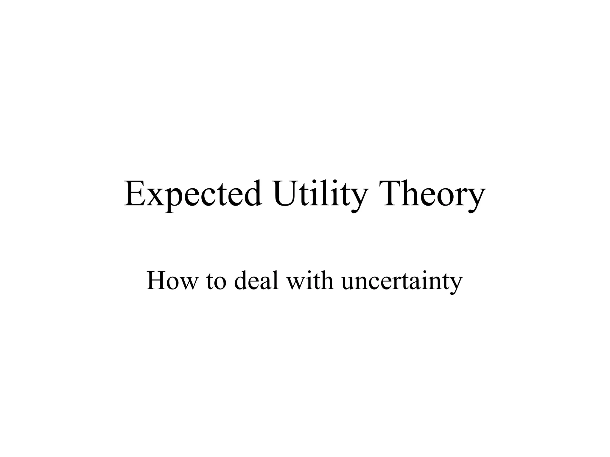
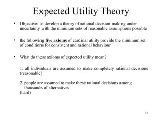
2 Goals
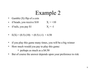
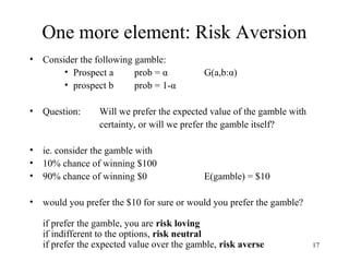
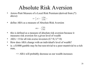
1) Individual maximizes their expected Utility
0.4
0.6
0.3
0.7
10
2
9
4
Asset i
Asset j
E(W) = 0.4(10) + 0.6(2) = 5.2
E[U(W)] = 0.4U(10) + 0.6U(2) = ?
Prefer the one with higher E[U(W)]
E(W) = 0.3(9) + 0.7(4) = 5.5
E[U(W)] = 0.3U(9) + 0.7U(4) = ?
2) Individual preferences over risk and return
y
x
C2
C1
Return
Risk

4. 4
Probability
• probability of an event occurring is the relative
frequency with which the event occurs
• if αi = the probability of event i occurring and there
are n possible events (states) then
• 1. α> 0, i = 1…n
i • 2. å ‘i=1
α= 1
i • Lottery (X) with prizes (outcomes, states, events)
• X, X, X,...,Xwith corresponding probabilities
123n • α, α, α,...,α, respectively (mutually exclusive and
123n exhaustive)
• then the expected value of this lottery is
• E(X) = αXn
+ αX+ αX+ ... + αX11 22 33 nn
‘i=1
• E(X) = å αXii
n

5. 5
Example 1
• Gamble (X) flip of a coin
• if heads, you receive $1 X1 = +1
• if tails, you pay $1 X2 = -1
• E(X) = (0.5) (1) + (0.5) (-1) = 0
• if you play this game many times, it is likely that you
break-even

6. 6
Example 2
• Gamble (X) flip of a coin
• if heads, you receive $10 X1 = +10
• if tails, you pay $1 X2 = -1
• E(X) = (0.5) (10) + (0.5) (-1) = 4.50
• if you play this game many times, you will be a big winner
• How much would you pay to play this game:
• perhaps as much as a $4.50
• But of course the answer depends upon your preference to risk

7. 7
Fair Gambles
• if
the cost to play = expected value of
these gambles the outcome
– then the gamble is said to be actuarially fair
• Common empirical findings:
1. individuals may agree to flip a coin for small amounts of money,
but usually refuse to bet large sums of money
2. people will pay small amounts of money to play actuarially
unfair games (Lotto 649, where cost = $1, but E(X) < 1)
- but will avoid paying a lot
Why do these empirical findings occur? Becoz’ it is not about E(W)

8. 8
St. Petersburg Paradox
• Gamble (X):
• A coin is flipped until a head appears You receive $2n where n is the
flip on which the head occurred
• states: X1 = $2 X2 = $4 X3 = $8 ... Xn = $2n
• prob: α1 = 1/2 α2 = 1/4 α3 = 1/8 ... αn = 1/2n
E(X) =
1
å å å¥
a x
= i
= = ¥ i i i 2 1
2
=1
i
Paradox: no one would pay an “actuarially fair” price to play this game
(no one would even pay close to the fair price)

9. 9
Explaining the St. Petersburg Paradox
• this paradox arises because individuals do not make
decisions based purely on wealth, but rather on the utility
of their expected wealth
• if we can show that the marginal utility of wealth declines
as we get more wealth, then we can show that the expected
value of a game is finite
• Assume U(X) = ln(X) U'(X)=1/x > 0 MU positive
• U"(X)=-1/x2 < 0 Diminishing MU
¥ ¥
• E(U(W)) = E(S αi U(Xi)) = (S αi ln(Xi)) = 1.39 < ¥
‘i=1 ‘i=1
• an individual would pay an amount up to 1.39 units of
utility to play this gamble

10. 10
Expected Utility Theory
• Objective: to develop a theory of rational decision-making under
uncertainty with the minimum sets of reasonable assumptions possible
• the following five axioms of cardinal utility provide the minimum set
of conditions for consistent and rational behaviour
• What do these axioms of expected utility mean?
1. all individuals are assumed to make completely rational decisions
(reasonable)
2. people are assumed to make these rational decisions among
thousands of alternatives
(hard)

11. 5 Axioms of Choice under uncertainty
A1.Comparability (also known as completeness).
For the entire set of uncertain alternatives, an individual can say
either that
11
either x is preferred to outcome y (x > y)
or y is preferred to x (y > x)
or indifferent between x and y (x ~ y).
A2.Transitivity (also know as consistency).
If an individual prefers x to y and y to z, then x is preferred to z.
If (x > y and y > z, then x > z).
Similarly, if an individual is indifferent between x and y and is
also indifferent between y and z, then the individual is
indifferent between x and z. If (x ~ y and y ~ z, then x ~ z).

12. 5 Axioms of Choice under uncertainty
12
A3.Strong Independence.
Suppose we construct a gamble where the individual has a probability
α of receiving outcome x and a probability (1-α) of receiving outcome
z. This gamble is written as:
G(x,z:α)
Strong independence says that if the individual is indifferent to x and
y, then he will also be indifferent as to a first gamble set up between x
with probability α and a mutually exclusive outcome z, and a second
gamble set up between y with probability α and the same mutually
exclusive outcome z.
If x ~ y, then G(x,z:α) ~ G(y,z:α)
NOTE: The mutual exclusiveness of the third outcome z is critical to
the axiom of strong independence.

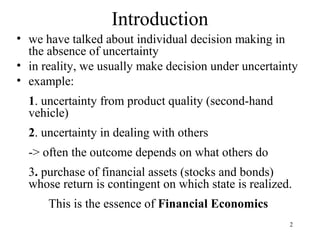
13. 5 Axioms of Choice under uncertainty
13
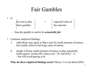
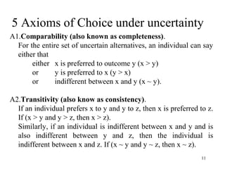
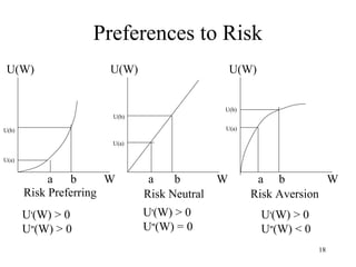
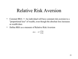
A4.Measurability. (CARDINAL UTILITY)
If outcome y is less preferred than x (y < x) but more than z (y > z),
then there is a unique probability α such that:
the individual will be indifferent between
[1] y and
[2] A gamble between x with probability α
z with probability (1-α).
In Maths,
if x > y > z or x > y > z ,
then there exists a unique α such that y ~ G(x,z:α)

14. 5 Axioms of Choice under uncertainty
14
A5.Ranking. (CARDINAL UTILITY)
If alternatives y and u both lie somewhere between x and
z and we can establish gambles such that an individual is
indifferent between y and a gamble between x (with probability α1)
and z, while also indifferent between u and a second gamble, this
time between x (with probability α2) and z, then if α1 is greater
than α2, y is preferred to u.
If x > y > z and x > u > z
then if y ~ G(x,z:α1) and u ~ G(x,z:α2),
then it follows that if α1 > α2 then y > u,
or if α1 = α2, then y ~ u

15. 15
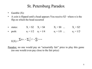
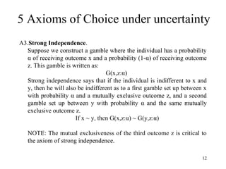
One more assumption
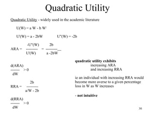
• People are greedy, prefer more wealth than
less.
• The 5 axioms and this assumption is all we
need in order to develop a expected utility
theorem and actually apply the rule of
max E[U(W)] = max ΣiαiU(Wi)

16. 16
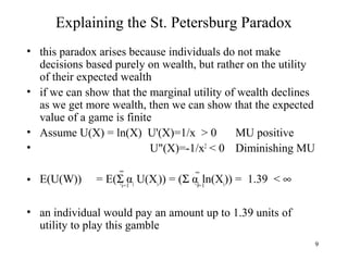
Utility Functions
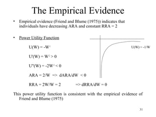
• Utility functions must have 2 properties
1. order preserving: if U(x) > U(y) => x > y
2. Expected utility can be used to rank combinations of risky
alternatives:
U[G(x,y:α)] = αU(x) + (1-α) U(y)
• Deriving Expected utility theorem, one of the most elegant derivations
in Economics, is tough. Don’t worry about a formal derivation. Just
apply it.
• Remark:
Utility functions are unique to individuals
- there is no way to compare one individual's utility function with
another individual's utility
- interpersonal comparisons of utility are impossible
if we give 2 people $1,000 there is no way to determine who is happier

17. 17
One more element: Risk Aversion
• Consider the following gamble:
• Prospect a prob = α G(a,b:α)
• prospect b prob = 1-α
• Question: Will we prefer the expected value of the gamble with
certainty, or will we prefer the gamble itself?
• ie. consider the gamble with
• 10% chance of winning $100
• 90% chance of winning $0 E(gamble) = $10
• would you prefer the $10 for sure or would you prefer the gamble?
if prefer the gamble, you are risk loving
if indifferent to the options, risk neutral
if prefer the expected value over the gamble, risk averse

18. U(b)
a b W a b W a b W
18
Preferences to Risk
U(W) U(W) U(W)
Risk Preferring Risk Neutral Risk Aversion
U(b)
U(a)
U'(W) > 0
U''(W) > 0
U'(W) > 0
U''(W) = 0
U'(W) > 0
U''(W) < 0
U(a)
U(b)
U(a)

19. 19
The Utility Function
U(W)
3.40
3.00
2.30
1.61
1 W 5 10 20 30
0
Let U(W) = ln(W)
U'(W) > 0
U''(W) < 0
U'(W) = 1/w
U''(W) = - 1/W2
MU positive
But diminishing

20. 20
U[E(W)] and E[U(W)]
• U[(E(W)] is the utility associated with the known
level of expected wealth (although there is
uncertainty around what the level of wealth will
be, there is no such uncertainty about its expected
value)
• E[U(W)] is the expected utility of wealth is utility
associated with level of wealth that may obtain
• The relationship between U[E(W)] and E[U(W)] is
very important

21. 21
Expected Utility
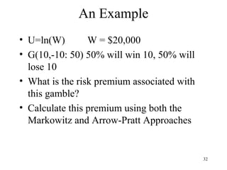
• Assume that the utility function is natural logs: U(W) = ln(W)
• Then MU(W) is decreasing
• U(W) = ln(W)
• U'(W)=1/W
• MU>0
• MU''(W) < 0 => MU diminishing
Consider the following example:
80% change of winning $5
20% chance of winning $30
E(W) = (.80)*(5) + (0.2)*(30) = $10
U[E(W)] = U(10) = 2.30
E[U(W)] = (0.8)*[U(5)] + (0.2)*[U(30)]
= (0.8)*(1.61) + (0.2)*(3.40)
= 1.97
Therefore, U[(E(W)] > E[U(W)] -- uncertainty reduces utility

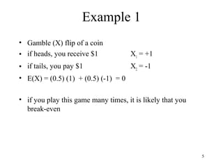
22. 22
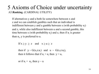
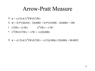
The Markowitz Premium
U(W)
3.40
1.61
1 W 5 10 30
U[E(W)] = 2.30
0
U[E(W)] = U(10) = 2.30
E[U(W)]
= 0.8*U(5) + 0.2*U(30)
= 0.8*1.61 + 0.2*3.40
= 1.97
Therefore, U[E(W)] > E[U(W)]
Uncertainty reduces utility
Certainty equivalent: 7.17
That is, this individual will take
7.17 with certainty rather than
the uncertainty around the gamble
CE
= 7.17
E[U(W)] = 1.97
2.83
U(W) = ln(W)

23. 23
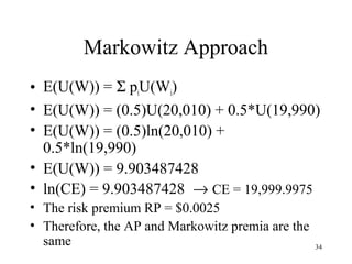
The Certainty Equivalent
• The Expected wealth is 10
• The E[U(W)] = 1.97
• How much would this individual take with
certainty and be indifferent the gamble
• Ln(CE) = 1.97
• Exp(Ln(CE)) = CE = 7.17
• This individual would take 7.17 with certainty
rather than the gamble with expected payoff of 10
• The difference, (10 – 7.17 ) = 2.83, can be viewed
as a risk premium – an amount that would be paid
to avoid risk

24. 24
The Risk Premium
• Risk Premium:
– the amount that the individual is willing to give up in order to avoid the
gamble
• Recall the gamble
80% change of winning $5
20% chance of winning $30
E(W) = (.80)*(5) + (0.2)*(30) = $10
Suppose the individual has the choice now between the gamble and the
expected value of the gamble
E[U[W)] = 1.97
Certainty equivalent = $7.17
Investor would be willing to pay a maximum of $2.83 to avoid the gamble
($10 - $7.17) ie will pay an insurance premium of $2.83.
THIS IS CALLED THE MARKOWITZ PREMIUM
Ln(CE)=1.97, i.e U(CE)=E[U(W)],, CE=7.17 RP=10-7.17=$2.83

25. 25
The Risk Premium
Risk
Premium
=
an individual's
expected
wealth,given he
plays the gamble
-
level of wealth the
individual would accept
with certainty if the
gamble were removed (ie
the certainty equivalent)
In general,
if U[E(W)] > E[U(W)] then risk averse individual (RP > 0)
if U[E(W)] = E[U(W)] then risk neutral individual (RP = 0)
if U[E(W)] < E[U(W)] then risk loving individual (RP < 0)
risk aversion occurs when the utility function is strictly concave
risk neutrality occurs when the utility function is linear
risk loving occurs when the utility function is convex

26. 26
The Arrow-Pratt Premium
• Risk Averse Investors
• assume that utility functions are strictly concave and increasing
• Individuals always prefer more to less (MU > 0)
• Marginal utility of wealth decreases as wealth increases
A More Specific Definition of Risk Aversion
W = current wealth
gamble Z and the gamble has a zero expected value
E(Z) = 0
what risk premium p(W,Z) must be added to the gamble to make the individual
indifferent between the gamble and the expected value of the gamble?

27. 27
The Arrow-Pratt Premium
The risk premium p can be defined as the value that satisfies the
following equation:
E[U(W + Z)] = U[ W + E(Z) - p( W , Z)] (*)
LHS: RHS:
expected utility of utility of the current level of wealth
the current level plus
of wealth, given the the expected value of
gamble the gamble
less
the risk premium
We want to use a Taylor series expansion to (*) to derive an expression
for the risk premium p(W,Z)

28. 28
Absolute Risk Aversion
• Arrow-Pratt Measure of a Local Risk Premium (derived from (*)
above)
)
¢¢
( - U (W)
p s
Z ¢
U (W)
= 1 2
2
• define ARA as a measure of Absolute Risk Aversion
¢¢
ARA = - U (W)
¢
U (W)
• this is defined as a measure of absolute risk aversion because it
measures risk aversion for a given level of wealth
• ARA > 0 for all risk averse investors (U'>0, U''<0)
• How does ARA change with an individual's level of wealth?
• ie. a $1000 gamble may be but non-trivial to a poor mantrivial to a rich
man,
=> ARA will probably decrease as our wealth increases

29. 29
Relative Risk Aversion
• Constant RRA => An individual will have constant risk aversion to a
"proportional loss" of wealth, even though the absolute loss increases
as wealth does
• Define RRA as a measure of Relative Risk Aversion
¢¢
RRA = - W*U (W)
¢
U (W)

30. 30
Quadratic Utility
Quadratic Utility - widely used in the academic literature
U(W) = a W - b W2
U'(W) = a - 2bW U"(W) = -2b
-U"(W) 2b
ARA = --------- = ---------
U'(W) a -2bW
d(ARA)
------- > 0
dW
2b
RRA = ---------
a/W - 2b
d(RRA)
------- > 0
dW
quadratic utility exhibits
increasing ARA
and increasing RRA
ie an individual with increasing RRA would
become more averse to a given percentage
loss in W as W increases
- not intuitive

31. 31
The Empirical Evidence
• Empirical evidence (Friend and Blume (1975)) indicates that
individuals have decreasing ARA and constant RRA = 2
• Power Utility Function
U(W) = -W-1
U'(W) = W-2 > 0
U"(W) = -2W-3 < 0
ARA = 2/W => dARA/dW < 0
RRA = 2W/W = 2 => dRRA/dW = 0
This power utility function is consistent with the empirical evidence of
Friend and Blume (1975)
U(W) = -1/W

32. 32
An Example
• U=ln(W) W = $20,000
• G(10,-10: 50) 50% will win 10, 50% will
lose 10
• What is the risk premium associated with
this gamble?
• Calculate this premium using both the
Markowitz and Arrow-Pratt Approaches

33. 33
Arrow-Pratt Measure
" p = -(1/2) s2
z U''(W)/U'(W)
" s2
z = 0.5*(20,010 – 20,000)2 + 0.5*(19,090 – 20,000)2 = 100
• U'(W) = (1/W) U''(W) = -1/W2
• U''(W)/U'(W) = -1/W = -1/(20,000)
" p = -(1/2) s2
z U''(W)/U'(W) = -(1/2)(100)(-1/20,000) = $0.0025

34. 34
Markowitz Approach
• E(U(W)) = S piU(Wi)
• E(U(W)) = (0.5)U(20,010) + 0.5*U(19,990)
• E(U(W)) = (0.5)ln(20,010) +
0.5*ln(19,990)
• E(U(W)) = 9.903487428
• ln(CE) = 9.903487428 ® CE = 19,999.9975
• The risk premium RP = $0.0025
• Therefore, the AP and Markowitz premia are the
same

35. 35
Markowitz Approach
19,990 20,000 20,010
CE
E(U(W))
= 9.903487

36. Differences in two approaches
• Markowitz premium is an exact measures whereas
the AP measure is approximate
• AP assumes symmetry payoffs across good or bad
states, as well as relatively small payoff changes.
• It is not always easy or even possible to invert a
utility function, in which case it is easier to
calculate the AP measure
• The accuracy of the AP measures decreases in the
size of the gamble and its asymmetry
36

37. 37
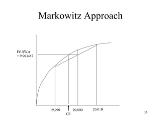
Mean & Variance as choice
variables
• With 5 axioms, prefer more to less, we
have Expected utility theorem
• With risk-aversion assumption, we
solve St. Petersburg’s paradox
• With returns of risky assets being
jointly normally distributed, we can
draw indifference curves on the plane
of return (E(r)) and risk (var(r) or
standard deviation of r) as the right
diagram
• Essentially, mean and variance are the
choice variables investors concern
about in order to max their E[U(w)]
Return
Risk