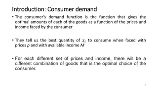
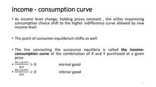
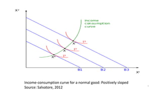
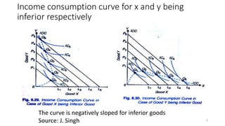
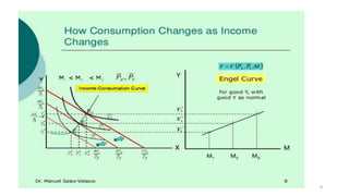
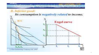
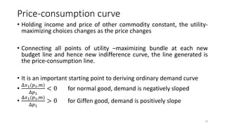
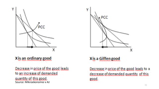
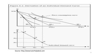
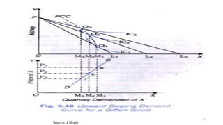
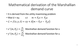
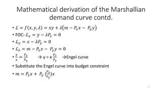
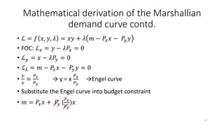
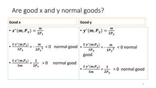
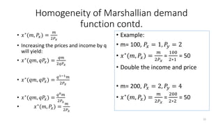
CONSUMER DEMAND
By
Linda Chinenyenwa Familusi
1
Outline
1. Introduction
2. Income-consumption curve
3. Engel curve
4. Price-consumption curve
5. Marshallian demand function
6. Indirect utility function
7. Roy’s identity
8. Market demand
9. Hicksian demand function
10. Expenditure function
11. Shephard Lemma
2
Introduction: Consumer demand
• The consumer’s demand function is the function that gives the
optimal amounts of each of the goods as a function of the prices and
income faced by the consumer
• They tell us the best quantity of 𝑥𝑖 to consume when faced with
prices p and with available income M
• For each different set of prices and income, there will be a
different combination of goods that is the optimal choice of the
consumer.
3
Income - consumption curve
• As income level change, holding prices constant , the utility maximizing
consumption choice shift to the higher indifference curve allowed by new
income level.
• The point of consumer equilibrium shifts as well
• The line connecting the successive equilibria is called the income-
consumption curve of the combination of X and Y purchased at a given
price
•
Δ𝑥1(𝑝,𝑚)
Δ𝑚
> 0 normal good
•
Δ𝑥1(𝑝.𝑚)
Δ𝑚
< 0 inferior good
4
Income-consumption curve for a normal good: Positively sloped
Source: Salvatore, 2012
5
Income consumption curve for x and y being
inferior respectively
6
The curve is negatively sloped for inferior goods
Source: J. Singh
Engel curve
• An Engel curve is a function relating the equilibrium quantity
purchased of a commodity to the level of money income
• Engel curve describes how quantity of Y changes as income changes
holding all prices constant
• It is derived from the income-consumption curve
7
8
9
Price-consumption curve
• Holding income and price of other commodity constant, the utility-
maximizing choices changes as the price changes
• Connecting all points of utility –maximizing bundle at each new
budget line and hence new indifference curve, the line generated is
the price-consumption line.
• It is an important starting point to deriving ordinary demand curve
•
Δ𝑥1(𝑝1,𝑚)
Δ𝑝1
< 0 for normal good, demand is negatively sloped
•
Δ𝑥1(𝑝1,𝑚)
Δ𝑝1
> 0 for Giffen good, demand is positively slope
10
11
Source: Mikroekonomie v AJ
Ordinary or Marshallian demand curve
• It is derived from the Price-consumption curve
• The Marshallian demand curve for a good relates equilibrium
quantities bought to the price of the good, assuming that all other
determinants are held constant
• A consumer’s Marshallian demand function specifies what the
consumer would buy in each price and wealth (or income), assuming
it perfectly solves the utility maximization problem
• Given the price-quantity relationship, the derived demand curve has
a negative slope for a normal good
12
13
Source: http://www.tutorhelpdesk.com
Positively sloped demand- Giffen good
• For a giffen good, the change in price and resulting change in the
quantity demanded moves in the same direction
• If the price of x falls, the position of the consumer equilibrium shifts
in such a way that the quantity of x decreases
• If the price of x rises, the position of the consumer equilibrium shifts
in such a way that the quantity of x increases
14
15
Source: J.Singh
Mathematical derivation of the Marshallian
demand curve
• It is derived from the utility maximizing problem
• Max U = xy; s.t 𝑚 = 𝑃𝑥 𝑥 + 𝑃𝑦y
• ℒ = 𝑓 𝑥, 𝑦, 𝜆 = 𝑥𝑦 + 𝜆 𝑚 − 𝑃𝑥 𝑥 − 𝑃𝑦 𝑦
• 𝑥∗(𝑚, 𝑃𝑥) =
𝑚
2𝑃 𝑥
Marshallian demand function for x
• 𝑦∗(𝑚, 𝑃𝑦) =
𝑚
2𝑃 𝑦
Marshallian demand function for y
16
Mathematical derivation of the Marshallian
demand curve contd.
• ℒ = 𝑓 𝑥, 𝑦, 𝜆 = 𝑥𝑦 + 𝜆 𝑚 − 𝑃𝑥 𝑥 − 𝑃𝑦 𝑦
• FOC: ℒ 𝑥 = 𝑦 − 𝜆𝑃𝑥 = 0
• ℒ 𝑦 = 𝑥 − 𝜆𝑃𝑦 = 0
• ℒ 𝜆 = 𝑚 − 𝑃𝑥 𝑥 − 𝑃𝑦 𝑦 = 0
•
𝑦
𝑥
=
𝑃 𝑥
𝑃 𝑦
→ y = x
𝑃 𝑥
𝑃 𝑦
→Engel curve
• Substitute the Engel curve into budget constraint
• 𝑚 = 𝑃𝑥 𝑥 + 𝑃𝑦 (
𝑃 𝑥
𝑃 𝑦
)𝑥
17
Mathematical derivation of the Marshallian
demand curve contd.
• ℒ = 𝑓 𝑥, 𝑦, 𝜆 = 𝑥𝑦 + 𝜆 𝑚 − 𝑃𝑥 𝑥 − 𝑃𝑦 𝑦
• FOC: ℒ 𝑥 = 𝑦 − 𝜆𝑃𝑥 = 0
• ℒ 𝑦 = 𝑥 − 𝜆𝑃𝑦 = 0
• ℒ 𝜆 = 𝑚 − 𝑃𝑥 𝑥 − 𝑃𝑦 𝑦 = 0
•
𝑦
𝑥
=
𝑃 𝑥
𝑃 𝑦
→ y = x
𝑃 𝑥
𝑃 𝑦
→Engel curve
• Substitute the Engel curve into budget constraint
• 𝑚 = 𝑃𝑥 𝑥 + 𝑃𝑦 (
𝑃 𝑥
𝑃 𝑦
)𝑥
18
Mathematical derivation of the Marshallian
demand curve contd.
• 𝑚 = 2 𝑃𝑥 𝑥
• The demand for good x will be:
• 𝒙∗(𝒎, 𝑷 𝒙) =
𝒎
𝟐𝑷 𝒙
Marshallian demand function for x
• Substituting the demand for x into the Engel curve, we get:
• y =
𝑚
2𝑃 𝑥
𝑃 𝑥
𝑃 𝑦
=
𝑚
2𝑃 𝑥
𝑃 𝑥
𝑃 𝑦
• 𝒚∗
(𝒎, 𝑷 𝒚) =
𝒎
𝟐𝑷 𝒚
Marshallian demand function for y
19
Are good x and y normal goods?
Good x
• 𝒙∗
(𝒎, 𝑷 𝒙) =
𝒎
𝟐𝑷 𝒙
•
δ 𝒙∗(𝒎,𝑷 𝒙)
δ𝑷 𝒙
= -
𝒎
𝟐𝑷 𝒙
𝟐 < 0 normal good
•
δ 𝒙∗(𝒎,𝑷 𝒙)
δ𝒎
=
𝟏
𝟐𝑷 𝒙
> 0 normal good
Good y
• 𝒚∗(𝒎, 𝑷 𝒚) =
𝒎
𝟐𝑷 𝒚
•
δ 𝒚∗(𝒎,𝑷 𝒚)
δ𝑷 𝒚
= -
𝒎
𝟐𝑷 𝒚
𝟐 < 0 normal
good
•
δ 𝒚∗(𝒎,𝑷 𝒚)
δ𝒎
=
𝟏
𝟐𝑷 𝒚
> 0 normal good
20
Homogeneity of Marshallian demand
function
• Marshallian demand function is homogenous of degree zero in price
and income
• Homogeneity of degrees zero implies that the price and income
derivatives of demand for a good, when weighted by prices and
income, sum up to zero
21
Homogeneity of Marshallian demand
function contd.
• 𝑥∗(𝑚, 𝑃𝑥) =
𝑚
2𝑃 𝑥
• Increasing the prices and income by q
will yield:
• 𝑥∗(𝑞𝑚, 𝑞𝑃𝑥) =
𝑞𝑚
2𝑞𝑃 𝑥
• 𝑥∗
(𝑞𝑚, 𝑞𝑃𝑥) =
𝑞1−1 𝑚
2𝑃𝑥
• 𝑥∗(𝑞𝑚, 𝑞𝑃𝑥) =
𝑞0 𝑚
2𝑃𝑥
• 𝑥∗(𝑚, 𝑃𝑥) =
𝑚
2𝑃𝑥
• Example:
• m= 100, 𝑃𝑥 = 1, 𝑃𝑦 = 2
• 𝑥∗
(𝑚, 𝑃𝑥) =
𝑚
2𝑃 𝑥
=
100
2∗1
= 50
• Double the income and price
• m= 200, 𝑃𝑥 = 2, 𝑃𝑦 = 4
• 𝑥∗(𝑚, 𝑃𝑥) =
𝑚
2𝑃 𝑥
=
200
2∗2
= 50
22
Indirect utility function
• The optimal level of utility obtainable will depend indirectly on the
prices of a good being bought and the individual’s income
• Consumers usually think about their preferences in terms of what
they consume rather than the prices
• To find the optimal solution, we substitute the Marshallian demand
functions in the utility function, the resulting utility function is called
the indirect utility function Ψ (𝑃1, 𝑃2, … , 𝑃𝑛,m)
23
Indirect utility function contd.
• u = xy
• Rem: 𝑥∗(𝑚, 𝑃𝑥) =
𝑚
2𝑃 𝑥
𝑦∗(𝑚, 𝑃𝑦) =
𝑚
2𝑃 𝑦
• U(𝑥𝑖 𝑝, 𝑚 = Ψ (𝑃1, 𝑃2, … , 𝑃𝑛,m)
• Ψ (𝑃1, 𝑃2, … , 𝑃𝑛,m) =
𝑚
2𝑃 𝑥
.
𝑚
2𝑃 𝑦
=
𝒎 𝟐
𝟒𝑷 𝒙 𝑷 𝒚
→ The indirect utility function
24
Properties of indirect utility function
• Non-increasing in prices
• Non-decreasing in income
• Homogenous to degree zero in price and income
• Quasi-convex in prices and income
25
Indirect utility function: Non-increasing in prices
and non-decreasing in income
•
𝒎 𝟐
𝟒𝑷 𝒙 𝑷 𝒚
=
𝟏
𝟒
𝒎 𝟐 𝒑 𝒙
−𝟏 𝒑 𝒚
−𝟏 → The indirect utility function
•
𝒅Ψ
𝒅𝒑 𝒙
= −
𝟏
𝟒
𝒎 𝟐 𝒑 𝒙
−𝟐 𝒑 𝒚
−𝟏 < 0 (1)
•
𝒅Ψ
𝒅𝒑 𝒚
= −
𝟏
𝟒
𝒎 𝟐
𝒑 𝒙
−𝟏
𝒑 𝒚
−𝟐
< 0 (2)
•
𝒅Ψ
𝒅𝒎
=
𝟏
𝟐
𝒎 𝒑 𝒙
−𝟏 𝒑 𝒚
−𝟏 > 0 (3)
• This is a valid indirect utility function
26
Indirect utility function: Quasi-convex in price and
income
•
𝒅 𝟐Ψ
𝒅𝒑 𝒙
𝟐 = 𝒇 𝒙𝒙 =
𝟏
𝟐
𝒎 𝟐 𝒑 𝒙
−𝟑 𝒑 𝒚
−𝟏 ≥ 0
• 𝒇 𝒙𝒚 =
𝟏
𝟒
𝒎 𝟐 𝒑 𝒙
−𝟐 𝒑 𝒚
−𝟐
•
𝒅 𝟐Ψ
𝒅𝒑 𝒚
𝟐 = 𝒇 𝒚𝒚 =
𝟏
𝟐
𝒎 𝟐 𝒑 𝒙
−𝟏 𝒑 𝒚
−𝟑 ≥ 0
• 𝒇 𝒚𝒙 =
𝟏
𝟒
𝒎 𝟐 𝒑 𝒙
−𝟐 𝒑 𝒚
−𝟐
•
𝒅 𝟐Ψ
𝒅𝒎 𝟐 =
𝟏
𝟐
𝒑 𝒙
−𝟏
𝒑 𝒚
−𝟏
≥ 0
• 𝒇 𝒙𝒙 𝒇 𝒚𝒚 - 𝒇 𝒙𝒚
𝟐
≤ 0
𝒎 𝟒
𝟒𝒑 𝒙
𝟒 𝒑 𝒚
𝟒 -
𝒎 𝟒
𝟏𝟔𝒑 𝒙
𝟒 𝒑 𝒚
𝟒 ≤ 0 (answer is close to zero i.e. 0.18)
• This is a valid indirect utility function
27
Indirect utility function: Homogenous to degree
zero in price and income
• Ψ (𝑃𝑥, 𝑃𝑦,m) =
𝒎 𝟐
𝟒𝑷 𝒙 𝑷 𝒚
→ The indirect utility function
• Ψ (q𝑃𝑥, q𝑃𝑦, 𝑞m) =
𝒒 𝟐 𝒎 𝟐
𝟒𝒒𝑷 𝒙 𝒒𝑷 𝒚
=
𝒒 𝟐 𝒎 𝟐
𝒒 𝟐 𝟒𝑷 𝒙 𝑷 𝒚
(q>0)
• Ψ (q𝑃𝑥, q𝑃𝑦, 𝑞m) =
𝒒 𝟐−𝟐 𝒎 𝟐
𝟒𝑷 𝒙 𝑷 𝒚
• Ψ (q𝑃𝑥, q𝑃𝑦, 𝑞m) =
𝒒 𝟎 𝒎 𝟐
𝟒𝑷 𝒙 𝑷 𝒚
• Ψ (𝑷 𝒙, 𝑷 𝒚,m) =
𝒎 𝟐
𝟒𝑷 𝒙 𝑷 𝒚
→ The indirect utility function
• This is a valid indirect utility function
28
Roy’s Identity for deriving Marshallian demand for
good x
• x(𝑃𝑥, 𝑃𝑦, 𝑚) = −
𝛿Ψ 𝛿𝑝 𝑥
𝛿Ψ 𝛿𝑚
• x(𝑃𝑥, 𝑃𝑦, 𝑚) = −
−𝟏
𝟒
𝒎 𝟐 𝒑 𝒙
−𝟐 𝒑 𝒚
−𝟏
𝟏
𝟐
𝒎 𝒑 𝒙
−𝟏 𝒑 𝒚
−𝟏
• x(𝑃𝑥, 𝑃𝑦, 𝑚) =
𝟏
𝟐
𝒎 𝟐−𝟏 𝒑 𝒙
−𝟐+𝟏 𝒑 𝒚
−𝟏+𝟏
• 𝒙∗(𝒎, 𝑷 𝒙) =
𝒎
𝟐𝑷 𝒙
Marshallian demand function for x
29
Roy’s Identity for deriving Marshallian demand for
good y
• y(𝑃𝑥, 𝑃𝑦, 𝑚) = −
𝛿Ψ 𝛿𝑝 𝑦
𝛿Ψ 𝛿𝑚
• y(𝑃𝑥, 𝑃𝑦, 𝑚) = −
−𝟏
𝟒
𝒎 𝟐 𝒑 𝒙
−𝟏 𝒑 𝒚
−𝟐
𝟏
𝟐
𝒎 𝒑 𝒙
−𝟏 𝒑 𝒚
−𝟏
• y(𝑃𝑥, 𝑃𝑦, 𝑚) =
𝟏
𝟐
𝒎 𝟐−𝟏 𝒑 𝒙
−𝟏+𝟏 𝒑 𝒚
−𝟐+𝟏
• 𝒚∗
(𝒎, 𝑷 𝒚) =
𝒎
𝟐𝑷 𝒚
Marshallian demand function for y
30
Market demand
• This is the aggregates of consumer demand
• It gives the total quantity demanded by all consumers at each prices,
holding total income and prices of other goods constant
• We assume that both individuals face the same prices and each person is a
price taker
• Each persons demand depends on her own income
• The demand is downward sloping
31
Market demand contd.
32Source: J. Singh
Shifts in the market demand curve
• The change in price will result in a movement along the market
demand curve
• Whereas change in other determinants of demand will result in a shift
in the marker demand curve to a new position
• Eg rise in income , rise in price of substitute
33
Shifts in the market demand curve
34
Hicksian demand or Compensated demand
function
• It finds the cheapest consumption bundle that achieves a given utility
level and measures the impact of price changes for fixed utility.
• Hicksian demand curve shows the relationship between the price of a
good and the quantity purchased on the assumption that other prices
and utility are held constant
35
Derivation of Hicksian demand or Compensated demand
function
36Source: www.slideshare.net
Mathematical derivation of Hicksian demand or
Compensated demand function
• min 𝐸 = 𝑃𝑥 𝑥 + 𝑃𝑦y
• s.t. U(x,y) = xy
• ℒ = 𝑓 𝑥, 𝑦, 𝜆 = 𝑃𝑥 𝑥 + 𝑃𝑦y + 𝜆 𝑢 − 𝑥𝑦
• FOC: ℒ 𝑥 = 𝑃𝑥 − 𝜆𝑦 = 0
• ℒ 𝑦 = 𝑃𝑦 − 𝜆𝑥 = 0
• ℒ 𝜆 = 𝑢 − 𝑥𝑦 = 0
•
𝑃 𝑥
𝑃 𝑦
=
𝑦
𝑥
→ y = x
𝑃 𝑥
𝑃 𝑦
→Engel curve
• Substitute the Engel curve into utility function
37
Hicksian demand or Compensated demand
function
• 𝑢 = 𝑥𝑦 → u = x(x
𝑃 𝑥
𝑃 𝑦
)
• u = 𝑥2(
𝑃 𝑥
𝑃 𝑦
) → 𝑥2 = u
𝑃 𝑦
𝑃𝑥
• Square root both sides: 𝑥2 = u
𝑃 𝑦
𝑃 𝑥
• 𝑥2 = u
𝑃 𝑦
𝑃 𝑥
• 𝒙 𝒄
∗(𝑷 𝒙, 𝑷 𝒚, 𝒖) =
𝑷 𝒚
𝑷 𝒙
𝒖 or
𝑷 𝒚
𝑷 𝒙
𝒖 𝟎.𝟓 Hicksian demand function for x
38
Hicksian demand or Compensated demand
function
• Substitute the Hicksian demand for x in the Engel curve: y = x
𝑃 𝑥
𝑃 𝑦
• y =
𝑃 𝑦
𝑃 𝑥
𝑢 0.5 𝑃𝑥
𝑃 𝑦
→ 𝑝 𝑦
0.5
𝑝 𝑥
−0.5
𝑝 𝑥
1
𝑝 𝑦
−1
𝑢0.5
• y =𝑝 𝑥
0.5
𝑝 𝑦
−0.5
𝑢0.5
• 𝑦𝑐
∗(𝑃𝑥, 𝑃𝑦, 𝑢) =
𝑃 𝑥
𝑃 𝑦
𝑢 or
𝑃 𝑥
𝑃 𝑦
𝑢 𝟎.𝟓 Hicksian demand function for y
39
Homogeneity of Hicksian demand function
• Hicksian demand function is homogenous of degree zero in price
• Increasing all prices by q:
• 𝑦𝑐
∗ 𝑞𝑃𝑥, 𝑞𝑃𝑦, 𝑢 =
𝑞𝑃𝑥
𝑞𝑃 𝑦
𝑢 0.5
• 𝑦𝑐
∗(𝑞𝑃𝑥, 𝑞𝑃𝑦, 𝑢) =
𝑞0.5
𝑞0.5
𝑃 𝑥
𝑃 𝑦
𝑢 0.5
• 𝑦𝑐
∗
(𝑞𝑃𝑥, 𝑞𝑃𝑦, 𝑢) = 𝑞0.5−0.5 𝑃 𝑥
𝑃 𝑦
𝑢 0.5
= 𝑞0 𝑃 𝑥
𝑃 𝑦
𝑢 0.5
• 𝑦𝑐
∗
(𝑃𝑥, 𝑃𝑦, 𝑢) =
𝑃𝑥
𝑃 𝑦
𝑢 or
𝑃𝑥
𝑃 𝑦
𝑢 0.5
Hicksian demand function for y
40
Expenditure function
• At optimal levels of utility, the consumer spends all the income at
disposal.
• Income = expenditure
• We allocate income in such a way as to achieve a given level of utility
with minimum expenditure for a particular set of prices
• To find the optimal solution, we substitute the Hicksian demand
functions into the expenditure function
41
Derivative of the expenditure function
• Substitute the Hicksian demand functions into the objective function:
m = 𝑃𝑥 𝑥 + 𝑃𝑦y → Expenditure equation
• Rem: 𝑥 𝑐
∗
(𝑃𝑥, 𝑃𝑦, 𝑢) =
𝑃 𝑦
𝑃 𝑥
𝑢 0.5
and 𝑦𝑐
∗
(𝑃𝑥, 𝑃𝑦, 𝑢) =
𝑃 𝑥
𝑃 𝑦
𝑢 0.5
• 𝑚∗ = 𝑃𝑥
𝑃 𝑦
𝑃 𝑥
𝑢 0.5 + 𝑃𝑦
𝑃 𝑥
𝑃 𝑦
𝑢 0.5
• Simplifying:
• 𝒎∗
= (𝟐 𝒖 𝟎.𝟓
𝒑 𝒙
𝟎.𝟓
𝒑 𝒚
𝟎.𝟓
) → The Expenditure function
• Or 𝒎∗=2( 𝒖 𝑷 𝒙 𝑷 𝒚) 𝟎.𝟓
42
Properties of expenditure function
1. e(p,u) is homogenous to degree one in price
2. e(p,u) is strictly increasing in u, and non-decreasing in price
3. e(p,u) is concave in price
43
Expenditure function: Homogenous to degree
one in price
• 𝒎∗=2( 𝒖 𝑷 𝒙 𝑷 𝒚) 𝟎.𝟓 → The Expenditure function
• Let the prices be increasing by q:
• 𝒎∗
( 𝒒𝑷 𝒙, 𝒒𝑷 𝒚, u) = 2( 𝒖 𝒒𝑷 𝒙 𝒒𝑷 𝒚) 𝟎.𝟓
• 𝒎∗( 𝒒𝑷 𝒙, 𝒒𝑷 𝒚, u) = 2( 𝒖 𝑷 𝒙 𝑷 𝒚) 𝟎.𝟓 𝒒 𝟎.𝟓+𝟎.𝟓
• 𝒎∗( 𝒖, 𝒒𝑷 𝒙 , 𝒒𝑷 𝒚) → The Expenditure function
• This is a valid expenditure function
44
Expenditure function: Increasing in u, and non-
decreasing in p
• 𝒎∗ = (𝟐 𝒖 𝟎.𝟓 𝒑 𝒙
𝟎.𝟓 𝒑 𝒚
𝟎.𝟓) → The Expenditure function
•
𝑑𝑚∗
𝑑𝑝 𝑥
= 𝑢0.5 𝑝 𝑥
−0.5 𝑝 𝑦
0.5 > 0 → Shephard lemma (4)
•
𝑑𝑚∗
𝑑𝑝 𝑦
= 𝑢0.5
𝑝 𝑥
0.5
𝑝 𝑦
−0.5
> 0 → Shephard lemma (5)
•
𝑑𝑚∗
𝑑 𝑢
= 𝑢−0.5 𝑝 𝑥
0.5 𝑝 𝑦
0.5 > 0 (6)
• This is a valid expenditure function
45
Expenditure function: Concave in p
•
𝒅 𝟐 𝒎∗
𝒅𝒑 𝒙
𝟐 = 𝒇 𝒙𝒙 = −𝟎. 𝟓 𝒖 𝟎.𝟓
𝒑 𝒙
−𝟏.𝟓
𝒑 𝒚
𝟎.𝟓
≤ 0
• 𝒇 𝒙𝒚 = 𝟎. 𝟓 𝒖 𝟎.𝟓
𝒑 𝒙
−𝟎.𝟓
𝒑 𝒚
−𝟎.𝟓
•
𝒅 𝟐 𝒎∗
𝒅𝒑 𝒚
𝟐 = 𝒇 𝒚𝒚 = −𝟎. 𝟓 𝒖 𝟎.𝟓
𝒑 𝒙
𝟎.𝟓
𝒑 𝒚
−𝟏.𝟓
≤ 0
• 𝒇 𝒚𝒙 = 𝟎. 𝟓 𝒖 𝟎.𝟓
𝒑 𝒙
−𝟎.𝟓
𝒑 𝒚
−𝟎.𝟓
• 𝒇 𝒙𝒙 and 𝒇 𝒚𝒚 ≤ 0
• 𝒇 𝒙𝒙 𝒇 𝒚𝒚 − 𝒇 𝒙𝒚
𝟐
≥ 0
•
𝒖
𝟒𝒑 𝒙 𝒑 𝒚
-
𝒖
𝟒𝒑 𝒙 𝒑 𝒚
≥ 0 This is a valid expenditure function
46
Relationship between the indirect utility function
and the expenditure function
• Ψ (𝑃1, 𝑃2, … , 𝑃𝑛,m) = u =
𝑚2
4𝑃 𝑥 𝑃 𝑦
→ The indirect utility function
• Rearrange to make m the subject:
• 𝑚2= 𝑢4𝑃𝑥 𝑃𝑦
• Square root both sides
• 𝑚∗(𝑃𝑥, 𝑃𝑦, 𝑢)= (2 𝑢0.5 𝑝 𝑥
0.5 𝑝 𝑦
0.5) → The Expenditure function
• Or 𝑚∗
=2( 𝑢 𝑃𝑥 𝑃𝑦)0.5
47
Shephard Lemma
•
𝛿𝑚(𝑝 𝑥,,𝑝 𝑦,𝑢)
𝛿𝑝 𝑥
= 𝑥 𝑐
(𝑝 𝑥, 𝑝 𝑦, 𝑢) →
2 𝑢0.5 𝑝 𝑥
0.5 𝑝 𝑦
0.5
𝛿𝑝 𝑥
→ Shephard lemma
• 𝑥 𝑐
(𝑝 𝑥, 𝑝 𝑦, 𝑢) = 𝑢0.5
𝑝 𝑥
−0.5
𝑝 𝑦
0.5
• 𝑥 𝑐
∗(𝑃𝑥, 𝑃𝑦, 𝑢) =
𝑃 𝑦
𝑃 𝑥
𝑢 or
𝑃 𝑦
𝑃 𝑥
𝑢 0.5 Hicksian demand function for x
•
𝛿𝐸(𝑝 𝑥,,𝑝 𝑦,𝑢)
𝛿𝑝 𝑦
= 𝑦 𝑐(𝑝 𝑥,, 𝑝 𝑦, 𝑢) →
2 𝑢0.5 𝑝 𝑥
0.5 𝑝 𝑦
0.5
𝛿𝑝 𝑦
→ Shephard lemma
• 𝑦 𝑐
(𝑝 𝑥, 𝑝 𝑦, 𝑢) = 𝑢0.5
𝑝 𝑥
0.5
𝑝 𝑦
−0.5
• 𝑦𝑐
∗(𝑃𝑥, 𝑃𝑦, 𝑢) =
𝑃 𝑥
𝑃 𝑦
𝑢 or
𝑃 𝑥
𝑃 𝑦
𝑢 0.5 Hicksian demand function for y
48
Comparison between the Marshallian and Hicksian
demand function
Marshallian demand function
• It’s a function of p and m
• Measures the changes in
demand when income is held
constant
• Measures the total effect
Hicksian demand function
• It’s a function of p and u
• Measures the changes in
demand when utility is held
constant.
• Measures the change in demand
along an indifference curve
• Measures the substitution effect
49
Marshallian effect – Hicksian effect = income effect .
This is the difference between the two demand function
Further reading
• Practical approach to microeconomic theory: For graduate students in
Applied economics
• Varian, H.R. (2010).Intermediate microeconomics: A modern approach (8th
ed.). New York: W.W Norton & Company, Inc.
• Varian, H.R. (1992).Microeconomic analysis (3rd ed.). New York: W.W
Norton & Company, Inc.
• Wainwright, K.J. (2013).Marshall and Hicks: Understanding the
• Salvatore, Dominick. Microeconomics (PDF). Archived from the
original (PDF) on October 20, 2012.ordinary and compensated demand
50
Thank you !!!
51

Consumer Demand

  • 1.
  • 2.
    Outline 1. Introduction 2. Income-consumptioncurve 3. Engel curve 4. Price-consumption curve 5. Marshallian demand function 6. Indirect utility function 7. Roy’s identity 8. Market demand 9. Hicksian demand function 10. Expenditure function 11. Shephard Lemma 2
  • 3.
    Introduction: Consumer demand •The consumer’s demand function is the function that gives the optimal amounts of each of the goods as a function of the prices and income faced by the consumer • They tell us the best quantity of 𝑥𝑖 to consume when faced with prices p and with available income M • For each different set of prices and income, there will be a different combination of goods that is the optimal choice of the consumer. 3
  • 4.
    Income - consumptioncurve • As income level change, holding prices constant , the utility maximizing consumption choice shift to the higher indifference curve allowed by new income level. • The point of consumer equilibrium shifts as well • The line connecting the successive equilibria is called the income- consumption curve of the combination of X and Y purchased at a given price • Δ𝑥1(𝑝,𝑚) Δ𝑚 > 0 normal good • Δ𝑥1(𝑝.𝑚) Δ𝑚 < 0 inferior good 4
  • 5.
    Income-consumption curve fora normal good: Positively sloped Source: Salvatore, 2012 5
  • 6.
    Income consumption curvefor x and y being inferior respectively 6 The curve is negatively sloped for inferior goods Source: J. Singh
  • 7.
    Engel curve • AnEngel curve is a function relating the equilibrium quantity purchased of a commodity to the level of money income • Engel curve describes how quantity of Y changes as income changes holding all prices constant • It is derived from the income-consumption curve 7
  • 8.
  • 9.
  • 10.
    Price-consumption curve • Holdingincome and price of other commodity constant, the utility- maximizing choices changes as the price changes • Connecting all points of utility –maximizing bundle at each new budget line and hence new indifference curve, the line generated is the price-consumption line. • It is an important starting point to deriving ordinary demand curve • Δ𝑥1(𝑝1,𝑚) Δ𝑝1 < 0 for normal good, demand is negatively sloped • Δ𝑥1(𝑝1,𝑚) Δ𝑝1 > 0 for Giffen good, demand is positively slope 10
  • 11.
  • 12.
    Ordinary or Marshalliandemand curve • It is derived from the Price-consumption curve • The Marshallian demand curve for a good relates equilibrium quantities bought to the price of the good, assuming that all other determinants are held constant • A consumer’s Marshallian demand function specifies what the consumer would buy in each price and wealth (or income), assuming it perfectly solves the utility maximization problem • Given the price-quantity relationship, the derived demand curve has a negative slope for a normal good 12
  • 13.
  • 14.
    Positively sloped demand-Giffen good • For a giffen good, the change in price and resulting change in the quantity demanded moves in the same direction • If the price of x falls, the position of the consumer equilibrium shifts in such a way that the quantity of x decreases • If the price of x rises, the position of the consumer equilibrium shifts in such a way that the quantity of x increases 14
  • 15.
  • 16.
    Mathematical derivation ofthe Marshallian demand curve • It is derived from the utility maximizing problem • Max U = xy; s.t 𝑚 = 𝑃𝑥 𝑥 + 𝑃𝑦y • ℒ = 𝑓 𝑥, 𝑦, 𝜆 = 𝑥𝑦 + 𝜆 𝑚 − 𝑃𝑥 𝑥 − 𝑃𝑦 𝑦 • 𝑥∗(𝑚, 𝑃𝑥) = 𝑚 2𝑃 𝑥 Marshallian demand function for x • 𝑦∗(𝑚, 𝑃𝑦) = 𝑚 2𝑃 𝑦 Marshallian demand function for y 16
  • 17.
    Mathematical derivation ofthe Marshallian demand curve contd. • ℒ = 𝑓 𝑥, 𝑦, 𝜆 = 𝑥𝑦 + 𝜆 𝑚 − 𝑃𝑥 𝑥 − 𝑃𝑦 𝑦 • FOC: ℒ 𝑥 = 𝑦 − 𝜆𝑃𝑥 = 0 • ℒ 𝑦 = 𝑥 − 𝜆𝑃𝑦 = 0 • ℒ 𝜆 = 𝑚 − 𝑃𝑥 𝑥 − 𝑃𝑦 𝑦 = 0 • 𝑦 𝑥 = 𝑃 𝑥 𝑃 𝑦 → y = x 𝑃 𝑥 𝑃 𝑦 →Engel curve • Substitute the Engel curve into budget constraint • 𝑚 = 𝑃𝑥 𝑥 + 𝑃𝑦 ( 𝑃 𝑥 𝑃 𝑦 )𝑥 17
  • 18.
    Mathematical derivation ofthe Marshallian demand curve contd. • ℒ = 𝑓 𝑥, 𝑦, 𝜆 = 𝑥𝑦 + 𝜆 𝑚 − 𝑃𝑥 𝑥 − 𝑃𝑦 𝑦 • FOC: ℒ 𝑥 = 𝑦 − 𝜆𝑃𝑥 = 0 • ℒ 𝑦 = 𝑥 − 𝜆𝑃𝑦 = 0 • ℒ 𝜆 = 𝑚 − 𝑃𝑥 𝑥 − 𝑃𝑦 𝑦 = 0 • 𝑦 𝑥 = 𝑃 𝑥 𝑃 𝑦 → y = x 𝑃 𝑥 𝑃 𝑦 →Engel curve • Substitute the Engel curve into budget constraint • 𝑚 = 𝑃𝑥 𝑥 + 𝑃𝑦 ( 𝑃 𝑥 𝑃 𝑦 )𝑥 18
  • 19.
    Mathematical derivation ofthe Marshallian demand curve contd. • 𝑚 = 2 𝑃𝑥 𝑥 • The demand for good x will be: • 𝒙∗(𝒎, 𝑷 𝒙) = 𝒎 𝟐𝑷 𝒙 Marshallian demand function for x • Substituting the demand for x into the Engel curve, we get: • y = 𝑚 2𝑃 𝑥 𝑃 𝑥 𝑃 𝑦 = 𝑚 2𝑃 𝑥 𝑃 𝑥 𝑃 𝑦 • 𝒚∗ (𝒎, 𝑷 𝒚) = 𝒎 𝟐𝑷 𝒚 Marshallian demand function for y 19
  • 20.
    Are good xand y normal goods? Good x • 𝒙∗ (𝒎, 𝑷 𝒙) = 𝒎 𝟐𝑷 𝒙 • δ 𝒙∗(𝒎,𝑷 𝒙) δ𝑷 𝒙 = - 𝒎 𝟐𝑷 𝒙 𝟐 < 0 normal good • δ 𝒙∗(𝒎,𝑷 𝒙) δ𝒎 = 𝟏 𝟐𝑷 𝒙 > 0 normal good Good y • 𝒚∗(𝒎, 𝑷 𝒚) = 𝒎 𝟐𝑷 𝒚 • δ 𝒚∗(𝒎,𝑷 𝒚) δ𝑷 𝒚 = - 𝒎 𝟐𝑷 𝒚 𝟐 < 0 normal good • δ 𝒚∗(𝒎,𝑷 𝒚) δ𝒎 = 𝟏 𝟐𝑷 𝒚 > 0 normal good 20
  • 21.
    Homogeneity of Marshalliandemand function • Marshallian demand function is homogenous of degree zero in price and income • Homogeneity of degrees zero implies that the price and income derivatives of demand for a good, when weighted by prices and income, sum up to zero 21
  • 22.
    Homogeneity of Marshalliandemand function contd. • 𝑥∗(𝑚, 𝑃𝑥) = 𝑚 2𝑃 𝑥 • Increasing the prices and income by q will yield: • 𝑥∗(𝑞𝑚, 𝑞𝑃𝑥) = 𝑞𝑚 2𝑞𝑃 𝑥 • 𝑥∗ (𝑞𝑚, 𝑞𝑃𝑥) = 𝑞1−1 𝑚 2𝑃𝑥 • 𝑥∗(𝑞𝑚, 𝑞𝑃𝑥) = 𝑞0 𝑚 2𝑃𝑥 • 𝑥∗(𝑚, 𝑃𝑥) = 𝑚 2𝑃𝑥 • Example: • m= 100, 𝑃𝑥 = 1, 𝑃𝑦 = 2 • 𝑥∗ (𝑚, 𝑃𝑥) = 𝑚 2𝑃 𝑥 = 100 2∗1 = 50 • Double the income and price • m= 200, 𝑃𝑥 = 2, 𝑃𝑦 = 4 • 𝑥∗(𝑚, 𝑃𝑥) = 𝑚 2𝑃 𝑥 = 200 2∗2 = 50 22
  • 23.
    Indirect utility function •The optimal level of utility obtainable will depend indirectly on the prices of a good being bought and the individual’s income • Consumers usually think about their preferences in terms of what they consume rather than the prices • To find the optimal solution, we substitute the Marshallian demand functions in the utility function, the resulting utility function is called the indirect utility function Ψ (𝑃1, 𝑃2, … , 𝑃𝑛,m) 23
  • 24.
    Indirect utility functioncontd. • u = xy • Rem: 𝑥∗(𝑚, 𝑃𝑥) = 𝑚 2𝑃 𝑥 𝑦∗(𝑚, 𝑃𝑦) = 𝑚 2𝑃 𝑦 • U(𝑥𝑖 𝑝, 𝑚 = Ψ (𝑃1, 𝑃2, … , 𝑃𝑛,m) • Ψ (𝑃1, 𝑃2, … , 𝑃𝑛,m) = 𝑚 2𝑃 𝑥 . 𝑚 2𝑃 𝑦 = 𝒎 𝟐 𝟒𝑷 𝒙 𝑷 𝒚 → The indirect utility function 24
  • 25.
    Properties of indirectutility function • Non-increasing in prices • Non-decreasing in income • Homogenous to degree zero in price and income • Quasi-convex in prices and income 25
  • 26.
    Indirect utility function:Non-increasing in prices and non-decreasing in income • 𝒎 𝟐 𝟒𝑷 𝒙 𝑷 𝒚 = 𝟏 𝟒 𝒎 𝟐 𝒑 𝒙 −𝟏 𝒑 𝒚 −𝟏 → The indirect utility function • 𝒅Ψ 𝒅𝒑 𝒙 = − 𝟏 𝟒 𝒎 𝟐 𝒑 𝒙 −𝟐 𝒑 𝒚 −𝟏 < 0 (1) • 𝒅Ψ 𝒅𝒑 𝒚 = − 𝟏 𝟒 𝒎 𝟐 𝒑 𝒙 −𝟏 𝒑 𝒚 −𝟐 < 0 (2) • 𝒅Ψ 𝒅𝒎 = 𝟏 𝟐 𝒎 𝒑 𝒙 −𝟏 𝒑 𝒚 −𝟏 > 0 (3) • This is a valid indirect utility function 26
  • 27.
    Indirect utility function:Quasi-convex in price and income • 𝒅 𝟐Ψ 𝒅𝒑 𝒙 𝟐 = 𝒇 𝒙𝒙 = 𝟏 𝟐 𝒎 𝟐 𝒑 𝒙 −𝟑 𝒑 𝒚 −𝟏 ≥ 0 • 𝒇 𝒙𝒚 = 𝟏 𝟒 𝒎 𝟐 𝒑 𝒙 −𝟐 𝒑 𝒚 −𝟐 • 𝒅 𝟐Ψ 𝒅𝒑 𝒚 𝟐 = 𝒇 𝒚𝒚 = 𝟏 𝟐 𝒎 𝟐 𝒑 𝒙 −𝟏 𝒑 𝒚 −𝟑 ≥ 0 • 𝒇 𝒚𝒙 = 𝟏 𝟒 𝒎 𝟐 𝒑 𝒙 −𝟐 𝒑 𝒚 −𝟐 • 𝒅 𝟐Ψ 𝒅𝒎 𝟐 = 𝟏 𝟐 𝒑 𝒙 −𝟏 𝒑 𝒚 −𝟏 ≥ 0 • 𝒇 𝒙𝒙 𝒇 𝒚𝒚 - 𝒇 𝒙𝒚 𝟐 ≤ 0 𝒎 𝟒 𝟒𝒑 𝒙 𝟒 𝒑 𝒚 𝟒 - 𝒎 𝟒 𝟏𝟔𝒑 𝒙 𝟒 𝒑 𝒚 𝟒 ≤ 0 (answer is close to zero i.e. 0.18) • This is a valid indirect utility function 27
  • 28.
    Indirect utility function:Homogenous to degree zero in price and income • Ψ (𝑃𝑥, 𝑃𝑦,m) = 𝒎 𝟐 𝟒𝑷 𝒙 𝑷 𝒚 → The indirect utility function • Ψ (q𝑃𝑥, q𝑃𝑦, 𝑞m) = 𝒒 𝟐 𝒎 𝟐 𝟒𝒒𝑷 𝒙 𝒒𝑷 𝒚 = 𝒒 𝟐 𝒎 𝟐 𝒒 𝟐 𝟒𝑷 𝒙 𝑷 𝒚 (q>0) • Ψ (q𝑃𝑥, q𝑃𝑦, 𝑞m) = 𝒒 𝟐−𝟐 𝒎 𝟐 𝟒𝑷 𝒙 𝑷 𝒚 • Ψ (q𝑃𝑥, q𝑃𝑦, 𝑞m) = 𝒒 𝟎 𝒎 𝟐 𝟒𝑷 𝒙 𝑷 𝒚 • Ψ (𝑷 𝒙, 𝑷 𝒚,m) = 𝒎 𝟐 𝟒𝑷 𝒙 𝑷 𝒚 → The indirect utility function • This is a valid indirect utility function 28
  • 29.
    Roy’s Identity forderiving Marshallian demand for good x • x(𝑃𝑥, 𝑃𝑦, 𝑚) = − 𝛿Ψ 𝛿𝑝 𝑥 𝛿Ψ 𝛿𝑚 • x(𝑃𝑥, 𝑃𝑦, 𝑚) = − −𝟏 𝟒 𝒎 𝟐 𝒑 𝒙 −𝟐 𝒑 𝒚 −𝟏 𝟏 𝟐 𝒎 𝒑 𝒙 −𝟏 𝒑 𝒚 −𝟏 • x(𝑃𝑥, 𝑃𝑦, 𝑚) = 𝟏 𝟐 𝒎 𝟐−𝟏 𝒑 𝒙 −𝟐+𝟏 𝒑 𝒚 −𝟏+𝟏 • 𝒙∗(𝒎, 𝑷 𝒙) = 𝒎 𝟐𝑷 𝒙 Marshallian demand function for x 29
  • 30.
    Roy’s Identity forderiving Marshallian demand for good y • y(𝑃𝑥, 𝑃𝑦, 𝑚) = − 𝛿Ψ 𝛿𝑝 𝑦 𝛿Ψ 𝛿𝑚 • y(𝑃𝑥, 𝑃𝑦, 𝑚) = − −𝟏 𝟒 𝒎 𝟐 𝒑 𝒙 −𝟏 𝒑 𝒚 −𝟐 𝟏 𝟐 𝒎 𝒑 𝒙 −𝟏 𝒑 𝒚 −𝟏 • y(𝑃𝑥, 𝑃𝑦, 𝑚) = 𝟏 𝟐 𝒎 𝟐−𝟏 𝒑 𝒙 −𝟏+𝟏 𝒑 𝒚 −𝟐+𝟏 • 𝒚∗ (𝒎, 𝑷 𝒚) = 𝒎 𝟐𝑷 𝒚 Marshallian demand function for y 30
  • 31.
    Market demand • Thisis the aggregates of consumer demand • It gives the total quantity demanded by all consumers at each prices, holding total income and prices of other goods constant • We assume that both individuals face the same prices and each person is a price taker • Each persons demand depends on her own income • The demand is downward sloping 31
  • 32.
  • 33.
    Shifts in themarket demand curve • The change in price will result in a movement along the market demand curve • Whereas change in other determinants of demand will result in a shift in the marker demand curve to a new position • Eg rise in income , rise in price of substitute 33
  • 34.
    Shifts in themarket demand curve 34
  • 35.
    Hicksian demand orCompensated demand function • It finds the cheapest consumption bundle that achieves a given utility level and measures the impact of price changes for fixed utility. • Hicksian demand curve shows the relationship between the price of a good and the quantity purchased on the assumption that other prices and utility are held constant 35
  • 36.
    Derivation of Hicksiandemand or Compensated demand function 36Source: www.slideshare.net
  • 37.
    Mathematical derivation ofHicksian demand or Compensated demand function • min 𝐸 = 𝑃𝑥 𝑥 + 𝑃𝑦y • s.t. U(x,y) = xy • ℒ = 𝑓 𝑥, 𝑦, 𝜆 = 𝑃𝑥 𝑥 + 𝑃𝑦y + 𝜆 𝑢 − 𝑥𝑦 • FOC: ℒ 𝑥 = 𝑃𝑥 − 𝜆𝑦 = 0 • ℒ 𝑦 = 𝑃𝑦 − 𝜆𝑥 = 0 • ℒ 𝜆 = 𝑢 − 𝑥𝑦 = 0 • 𝑃 𝑥 𝑃 𝑦 = 𝑦 𝑥 → y = x 𝑃 𝑥 𝑃 𝑦 →Engel curve • Substitute the Engel curve into utility function 37
  • 38.
    Hicksian demand orCompensated demand function • 𝑢 = 𝑥𝑦 → u = x(x 𝑃 𝑥 𝑃 𝑦 ) • u = 𝑥2( 𝑃 𝑥 𝑃 𝑦 ) → 𝑥2 = u 𝑃 𝑦 𝑃𝑥 • Square root both sides: 𝑥2 = u 𝑃 𝑦 𝑃 𝑥 • 𝑥2 = u 𝑃 𝑦 𝑃 𝑥 • 𝒙 𝒄 ∗(𝑷 𝒙, 𝑷 𝒚, 𝒖) = 𝑷 𝒚 𝑷 𝒙 𝒖 or 𝑷 𝒚 𝑷 𝒙 𝒖 𝟎.𝟓 Hicksian demand function for x 38
  • 39.
    Hicksian demand orCompensated demand function • Substitute the Hicksian demand for x in the Engel curve: y = x 𝑃 𝑥 𝑃 𝑦 • y = 𝑃 𝑦 𝑃 𝑥 𝑢 0.5 𝑃𝑥 𝑃 𝑦 → 𝑝 𝑦 0.5 𝑝 𝑥 −0.5 𝑝 𝑥 1 𝑝 𝑦 −1 𝑢0.5 • y =𝑝 𝑥 0.5 𝑝 𝑦 −0.5 𝑢0.5 • 𝑦𝑐 ∗(𝑃𝑥, 𝑃𝑦, 𝑢) = 𝑃 𝑥 𝑃 𝑦 𝑢 or 𝑃 𝑥 𝑃 𝑦 𝑢 𝟎.𝟓 Hicksian demand function for y 39
  • 40.
    Homogeneity of Hicksiandemand function • Hicksian demand function is homogenous of degree zero in price • Increasing all prices by q: • 𝑦𝑐 ∗ 𝑞𝑃𝑥, 𝑞𝑃𝑦, 𝑢 = 𝑞𝑃𝑥 𝑞𝑃 𝑦 𝑢 0.5 • 𝑦𝑐 ∗(𝑞𝑃𝑥, 𝑞𝑃𝑦, 𝑢) = 𝑞0.5 𝑞0.5 𝑃 𝑥 𝑃 𝑦 𝑢 0.5 • 𝑦𝑐 ∗ (𝑞𝑃𝑥, 𝑞𝑃𝑦, 𝑢) = 𝑞0.5−0.5 𝑃 𝑥 𝑃 𝑦 𝑢 0.5 = 𝑞0 𝑃 𝑥 𝑃 𝑦 𝑢 0.5 • 𝑦𝑐 ∗ (𝑃𝑥, 𝑃𝑦, 𝑢) = 𝑃𝑥 𝑃 𝑦 𝑢 or 𝑃𝑥 𝑃 𝑦 𝑢 0.5 Hicksian demand function for y 40
  • 41.
    Expenditure function • Atoptimal levels of utility, the consumer spends all the income at disposal. • Income = expenditure • We allocate income in such a way as to achieve a given level of utility with minimum expenditure for a particular set of prices • To find the optimal solution, we substitute the Hicksian demand functions into the expenditure function 41
  • 42.
    Derivative of theexpenditure function • Substitute the Hicksian demand functions into the objective function: m = 𝑃𝑥 𝑥 + 𝑃𝑦y → Expenditure equation • Rem: 𝑥 𝑐 ∗ (𝑃𝑥, 𝑃𝑦, 𝑢) = 𝑃 𝑦 𝑃 𝑥 𝑢 0.5 and 𝑦𝑐 ∗ (𝑃𝑥, 𝑃𝑦, 𝑢) = 𝑃 𝑥 𝑃 𝑦 𝑢 0.5 • 𝑚∗ = 𝑃𝑥 𝑃 𝑦 𝑃 𝑥 𝑢 0.5 + 𝑃𝑦 𝑃 𝑥 𝑃 𝑦 𝑢 0.5 • Simplifying: • 𝒎∗ = (𝟐 𝒖 𝟎.𝟓 𝒑 𝒙 𝟎.𝟓 𝒑 𝒚 𝟎.𝟓 ) → The Expenditure function • Or 𝒎∗=2( 𝒖 𝑷 𝒙 𝑷 𝒚) 𝟎.𝟓 42
  • 43.
    Properties of expenditurefunction 1. e(p,u) is homogenous to degree one in price 2. e(p,u) is strictly increasing in u, and non-decreasing in price 3. e(p,u) is concave in price 43
  • 44.
    Expenditure function: Homogenousto degree one in price • 𝒎∗=2( 𝒖 𝑷 𝒙 𝑷 𝒚) 𝟎.𝟓 → The Expenditure function • Let the prices be increasing by q: • 𝒎∗ ( 𝒒𝑷 𝒙, 𝒒𝑷 𝒚, u) = 2( 𝒖 𝒒𝑷 𝒙 𝒒𝑷 𝒚) 𝟎.𝟓 • 𝒎∗( 𝒒𝑷 𝒙, 𝒒𝑷 𝒚, u) = 2( 𝒖 𝑷 𝒙 𝑷 𝒚) 𝟎.𝟓 𝒒 𝟎.𝟓+𝟎.𝟓 • 𝒎∗( 𝒖, 𝒒𝑷 𝒙 , 𝒒𝑷 𝒚) → The Expenditure function • This is a valid expenditure function 44
  • 45.
    Expenditure function: Increasingin u, and non- decreasing in p • 𝒎∗ = (𝟐 𝒖 𝟎.𝟓 𝒑 𝒙 𝟎.𝟓 𝒑 𝒚 𝟎.𝟓) → The Expenditure function • 𝑑𝑚∗ 𝑑𝑝 𝑥 = 𝑢0.5 𝑝 𝑥 −0.5 𝑝 𝑦 0.5 > 0 → Shephard lemma (4) • 𝑑𝑚∗ 𝑑𝑝 𝑦 = 𝑢0.5 𝑝 𝑥 0.5 𝑝 𝑦 −0.5 > 0 → Shephard lemma (5) • 𝑑𝑚∗ 𝑑 𝑢 = 𝑢−0.5 𝑝 𝑥 0.5 𝑝 𝑦 0.5 > 0 (6) • This is a valid expenditure function 45
  • 46.
    Expenditure function: Concavein p • 𝒅 𝟐 𝒎∗ 𝒅𝒑 𝒙 𝟐 = 𝒇 𝒙𝒙 = −𝟎. 𝟓 𝒖 𝟎.𝟓 𝒑 𝒙 −𝟏.𝟓 𝒑 𝒚 𝟎.𝟓 ≤ 0 • 𝒇 𝒙𝒚 = 𝟎. 𝟓 𝒖 𝟎.𝟓 𝒑 𝒙 −𝟎.𝟓 𝒑 𝒚 −𝟎.𝟓 • 𝒅 𝟐 𝒎∗ 𝒅𝒑 𝒚 𝟐 = 𝒇 𝒚𝒚 = −𝟎. 𝟓 𝒖 𝟎.𝟓 𝒑 𝒙 𝟎.𝟓 𝒑 𝒚 −𝟏.𝟓 ≤ 0 • 𝒇 𝒚𝒙 = 𝟎. 𝟓 𝒖 𝟎.𝟓 𝒑 𝒙 −𝟎.𝟓 𝒑 𝒚 −𝟎.𝟓 • 𝒇 𝒙𝒙 and 𝒇 𝒚𝒚 ≤ 0 • 𝒇 𝒙𝒙 𝒇 𝒚𝒚 − 𝒇 𝒙𝒚 𝟐 ≥ 0 • 𝒖 𝟒𝒑 𝒙 𝒑 𝒚 - 𝒖 𝟒𝒑 𝒙 𝒑 𝒚 ≥ 0 This is a valid expenditure function 46
  • 47.
    Relationship between theindirect utility function and the expenditure function • Ψ (𝑃1, 𝑃2, … , 𝑃𝑛,m) = u = 𝑚2 4𝑃 𝑥 𝑃 𝑦 → The indirect utility function • Rearrange to make m the subject: • 𝑚2= 𝑢4𝑃𝑥 𝑃𝑦 • Square root both sides • 𝑚∗(𝑃𝑥, 𝑃𝑦, 𝑢)= (2 𝑢0.5 𝑝 𝑥 0.5 𝑝 𝑦 0.5) → The Expenditure function • Or 𝑚∗ =2( 𝑢 𝑃𝑥 𝑃𝑦)0.5 47
  • 48.
    Shephard Lemma • 𝛿𝑚(𝑝 𝑥,,𝑝𝑦,𝑢) 𝛿𝑝 𝑥 = 𝑥 𝑐 (𝑝 𝑥, 𝑝 𝑦, 𝑢) → 2 𝑢0.5 𝑝 𝑥 0.5 𝑝 𝑦 0.5 𝛿𝑝 𝑥 → Shephard lemma • 𝑥 𝑐 (𝑝 𝑥, 𝑝 𝑦, 𝑢) = 𝑢0.5 𝑝 𝑥 −0.5 𝑝 𝑦 0.5 • 𝑥 𝑐 ∗(𝑃𝑥, 𝑃𝑦, 𝑢) = 𝑃 𝑦 𝑃 𝑥 𝑢 or 𝑃 𝑦 𝑃 𝑥 𝑢 0.5 Hicksian demand function for x • 𝛿𝐸(𝑝 𝑥,,𝑝 𝑦,𝑢) 𝛿𝑝 𝑦 = 𝑦 𝑐(𝑝 𝑥,, 𝑝 𝑦, 𝑢) → 2 𝑢0.5 𝑝 𝑥 0.5 𝑝 𝑦 0.5 𝛿𝑝 𝑦 → Shephard lemma • 𝑦 𝑐 (𝑝 𝑥, 𝑝 𝑦, 𝑢) = 𝑢0.5 𝑝 𝑥 0.5 𝑝 𝑦 −0.5 • 𝑦𝑐 ∗(𝑃𝑥, 𝑃𝑦, 𝑢) = 𝑃 𝑥 𝑃 𝑦 𝑢 or 𝑃 𝑥 𝑃 𝑦 𝑢 0.5 Hicksian demand function for y 48
  • 49.
    Comparison between theMarshallian and Hicksian demand function Marshallian demand function • It’s a function of p and m • Measures the changes in demand when income is held constant • Measures the total effect Hicksian demand function • It’s a function of p and u • Measures the changes in demand when utility is held constant. • Measures the change in demand along an indifference curve • Measures the substitution effect 49 Marshallian effect – Hicksian effect = income effect . This is the difference between the two demand function
  • 50.
    Further reading • Practicalapproach to microeconomic theory: For graduate students in Applied economics • Varian, H.R. (2010).Intermediate microeconomics: A modern approach (8th ed.). New York: W.W Norton & Company, Inc. • Varian, H.R. (1992).Microeconomic analysis (3rd ed.). New York: W.W Norton & Company, Inc. • Wainwright, K.J. (2013).Marshall and Hicks: Understanding the • Salvatore, Dominick. Microeconomics (PDF). Archived from the original (PDF) on October 20, 2012.ordinary and compensated demand 50
  • 51.