Download as PDF, PPTX

![Intermediate
microeconomics:
Lecture 2
Risk and Expected
utility
Risk attitude
Application to
insurance market
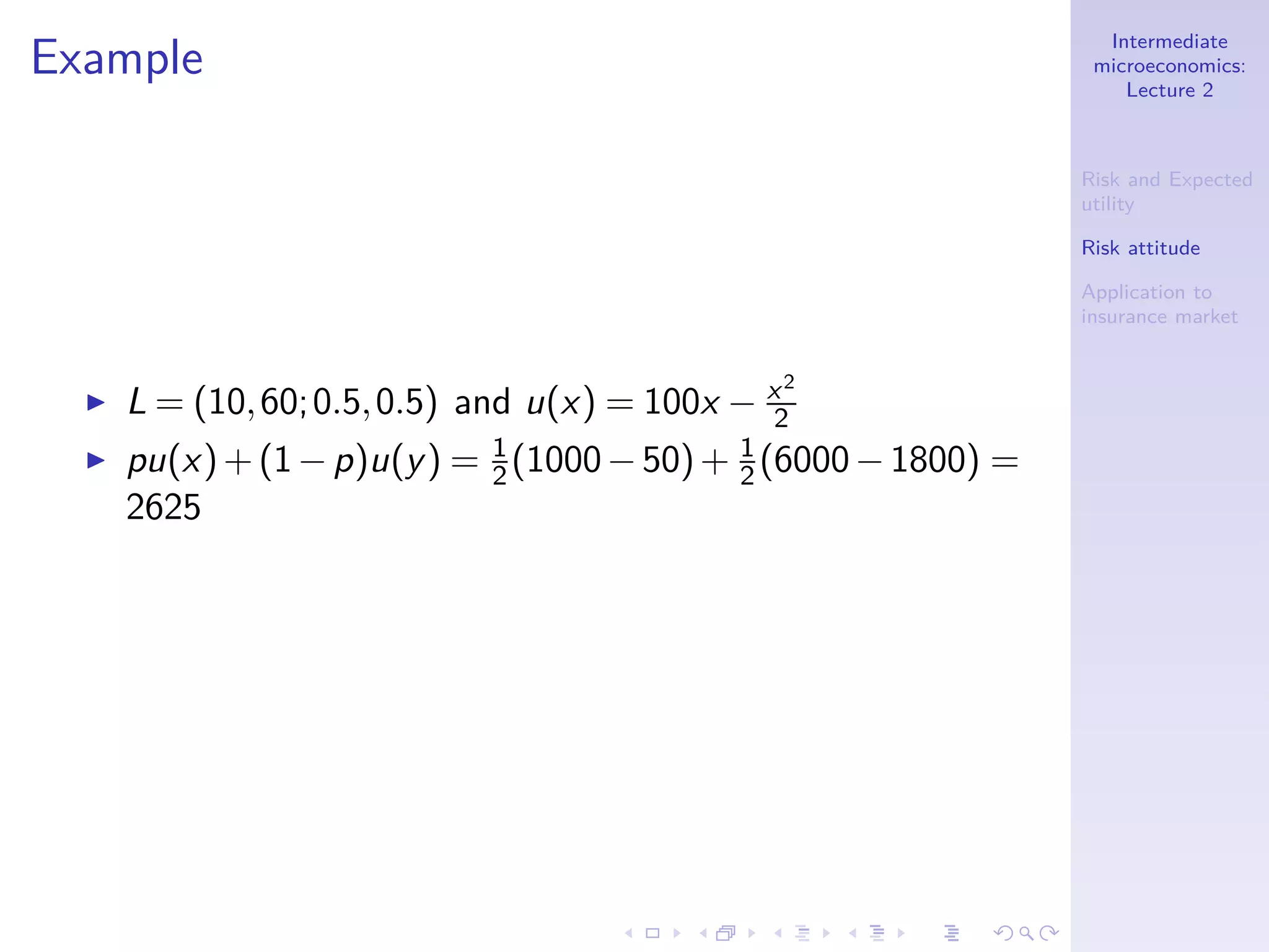
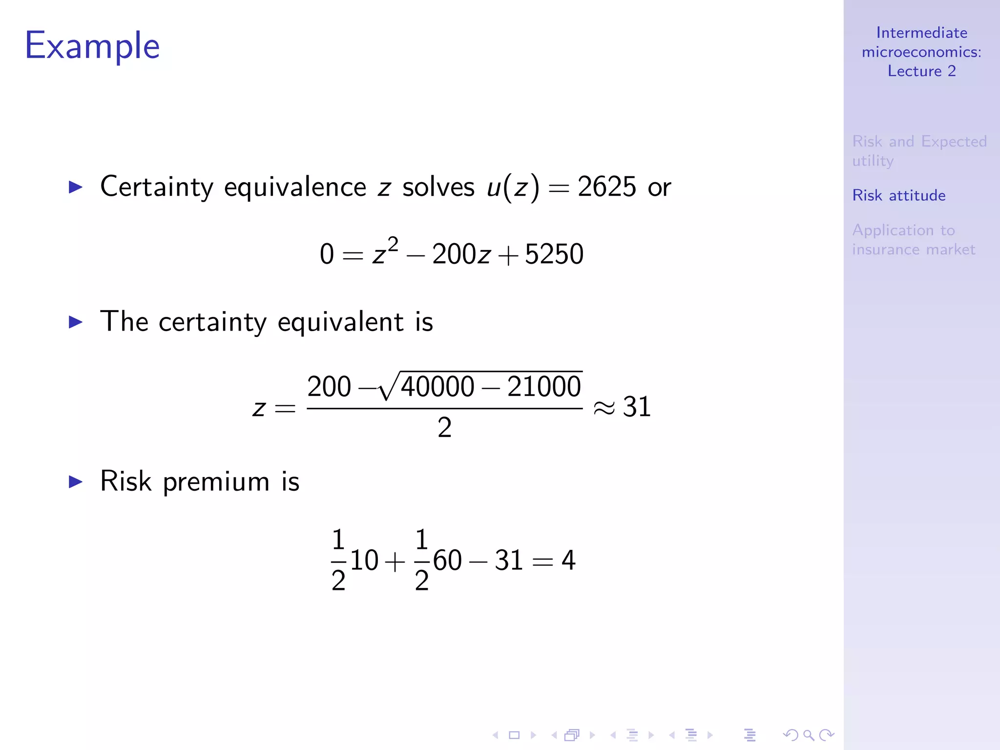
Example
◮ Suppose you cast a dice. If your get x ∈ {1,2,..,6}, you
receives $x.
◮ The expected utility is
EU(x) =
1
6
[u(1)+u(2)+u(3)+u(4)+u(5)+u(6)]
◮ For example, if u(x) =
√
x, then EU(x) = 1.805303682](https://image.slidesharecdn.com/lecture2-130420210559-phpapp01/75/Lecture-2-10-2048.jpg)
![Intermediate
microeconomics:
Lecture 2
Risk and Expected
utility
Risk attitude
Application to
insurance market
Independence
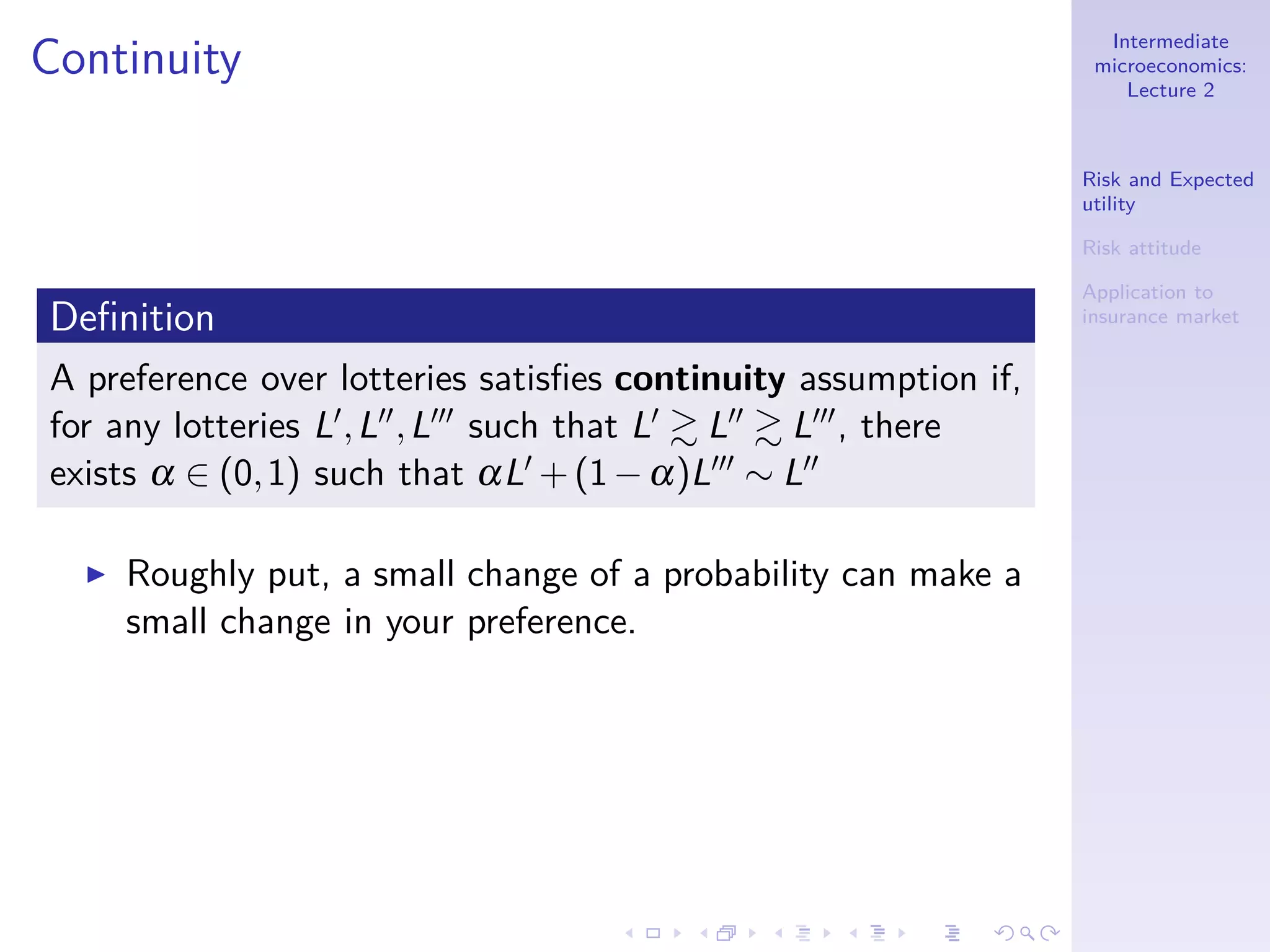
Definition
A preference over lotteries satisfies independence
assumption if, for any lotteries L′,L′′,L′′′ such that L′ L′′,
αL′ +(1−α)L′′′ αL′′ +(1−α)L′′′ for any α ∈ (0,1].
◮ Roughly put, if you expand two lotteries with a common
lottery, it should not affect preference over the two
lotteries.](https://image.slidesharecdn.com/lecture2-130420210559-phpapp01/75/Lecture-2-13-2048.jpg)
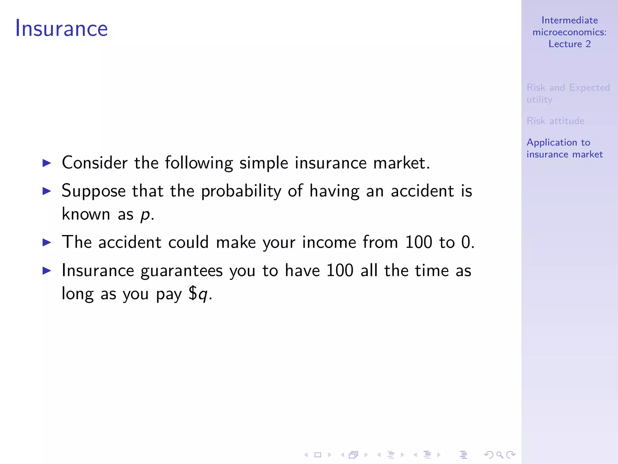
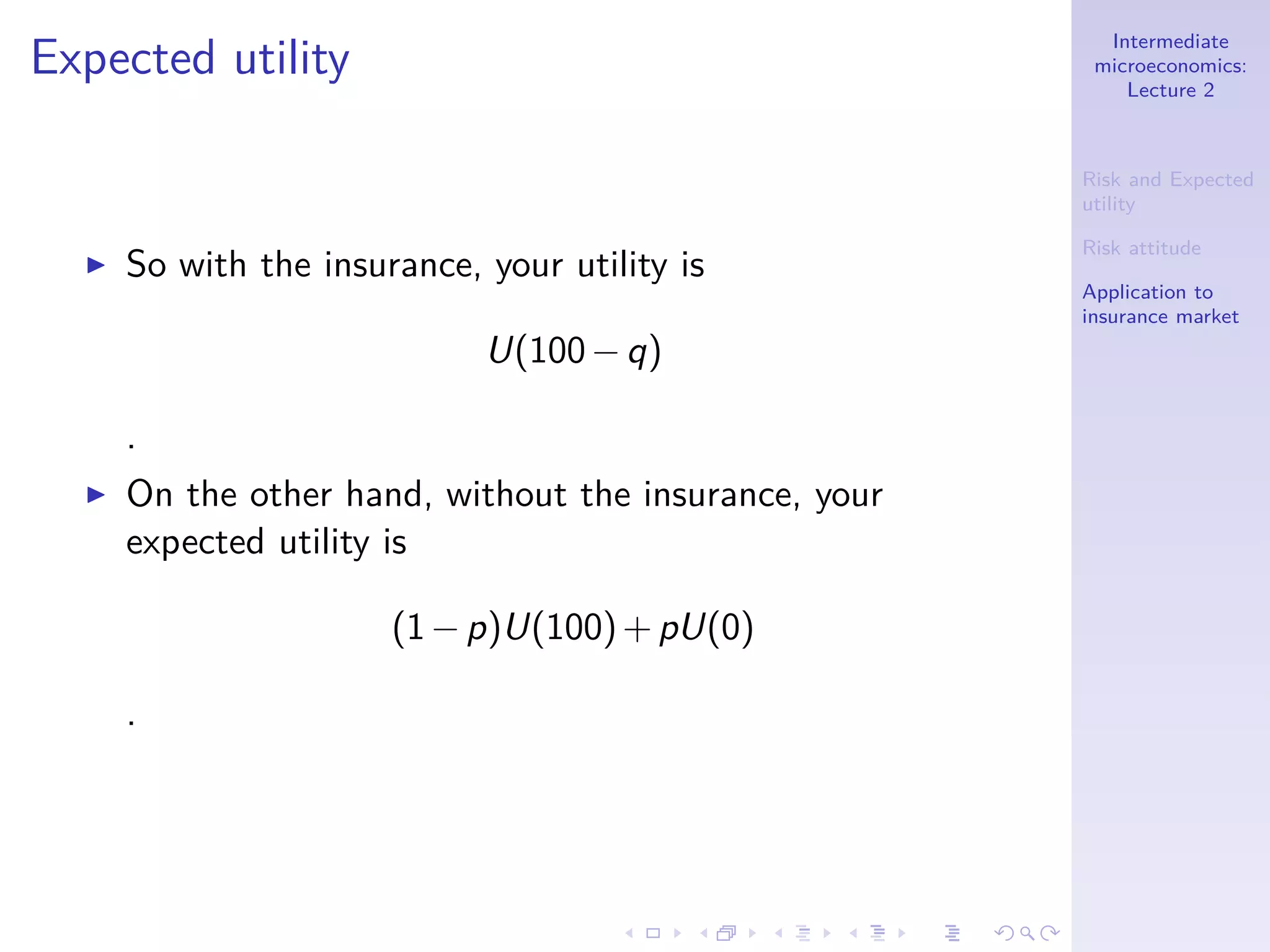

This document summarizes key points from Lecture 2 of an Intermediate Microeconomics course. It introduces risk and expected utility, defines risk attitudes like risk aversion and risk neutrality, and discusses how expected utility theory can represent preferences over risky outcomes. It also provides an example of how insurance markets work based on individuals' risk attitudes and the incentives of insurance companies.


