Stochastic Control/Reinforcement Learning for Optimal Market Making

Stochastic Control for Optimal Market-Making
Ashwin Rao
ICME, Stanford University
December 25, 2019
Ashwin Rao (Stanford) Optimal Market-Making December 25, 2019 1 / 30

Overview
1 Trading Order Book Dynamics
2 Deﬁnition of Optimal Market-Making Problem
3 Derivation of Avellaneda-Stoikov Analytical Solution
4 Real-world Optimal Market-Making and Reinforcement Learning

Trading Order Book (TOB)

Basics of Trading Order Book (TOB)
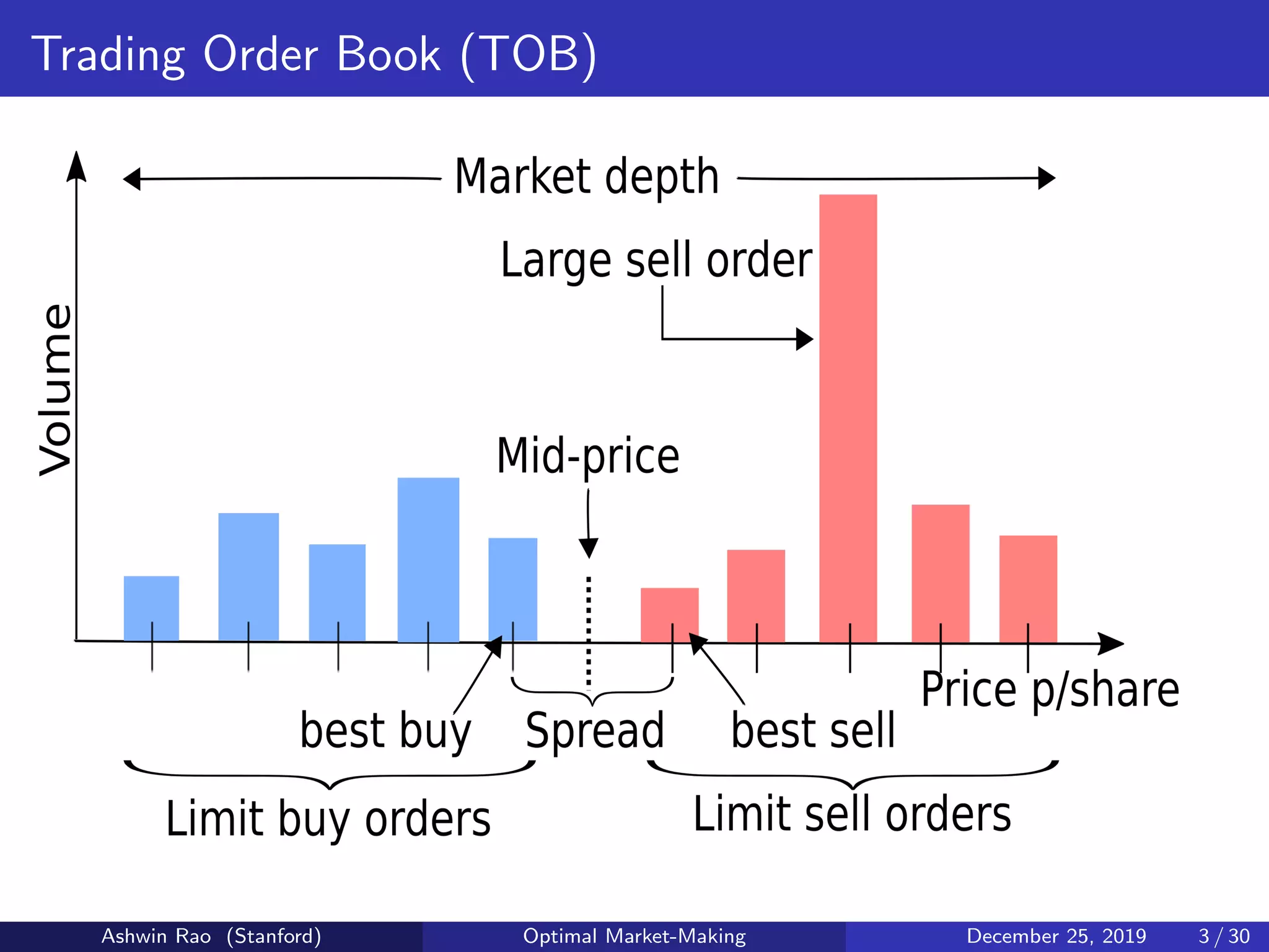
Buyers/Sellers express their intent to trade by submitting bids/asks
These are Limit Orders (LO) with a price P and size N
Buy LO (P,N) states willingness to buy N shares at a price ≤ P
Sell LO (P,N) states willingness to sell N shares at a price ≥ P
Trading Order Book aggregates order sizes for each unique price
So we can represent with two sorted lists of (Price, Size) pairs
Bids: [(P
(b)
i ,N
(b)
i ) 1 ≤ i ≤ m],P
(b)
i > P
(b)
j for i < j
Asks: [(P
(a)
i ,N
(a)
i ) 1 ≤ i ≤ n],P
(a)
i < P
(a)
j for i < j
We call P
(b)
1 as simply Bid, P
(a)
1 as Ask,
P
(a)
1 +P
(b)
1
2 as Mid
We call P
(a)
1 − P
(b)
1 as Spread, P
(a)
n − P
(b)
m as Market Depth
A Market Order (MO) states intent to buy/sell N shares at the best
possible price(s) available on the TOB at the time of MO submission

Trading Order Book (TOB) Activity
A new Sell LO (P,N) potentially removes best bid prices on the TOB
Removal: [(P
(b)
i ,min(N
(b)
i ,max(0,N −
i−1
∑
j=1
N
(b)
j ))) (i P
(b)
i ≥ P)]
After this removal, it adds the following to the asks side of the TOB
(P,max(0,N − ∑
i P
(b)
i ≥P
N
(b)
i ))
A new Buy MO operates analogously (on the other side of the TOB)
A Sell Market Order N will remove the best bid prices on the TOB
Removal: [(P
(b)
i ,min(N
(b)
i ,max(0,N −
i−1
∑
j=1
N
(b)
j ))) 1 ≤ i ≤ m]
A Buy Market Order N will remove the best ask prices on the TOB
Removal: [(P
(a)
i ,min(N
(a)
i ,max(0,N −
i−1
∑
j=1
N
(a)
j ))) 1 ≤ i ≤ n]

TOB Dynamics and Market-Making
Modeling TOB Dynamics involves predicting arrival of MOs and LOs
Market-makers are liquidity providers (providers of Buy and Sell LOs)
Other market participants are typically liquidity takers (MOs)
But there are also other market participants that trade with LOs
Complex interplay between market-makers & other mkt participants
Hence, TOB Dynamics tend to be quite complex
We view the TOB from the perspective of a single market-maker who
aims to gain with Buy/Sell LOs of appropriate width/size
By anticipating TOB Dynamics & dynamically adjusting Buy/Sell LOs
Goal is to maximize Utility of Gains at the end of a suitable horizon
If Buy/Sell LOs are too narrow, more frequent but small gains
If Buy/Sell LOs are too wide, less frequent but large gains
Market-maker also needs to manage potential unfavorable inventory
(long or short) buildup and consequent unfavorable liquidation

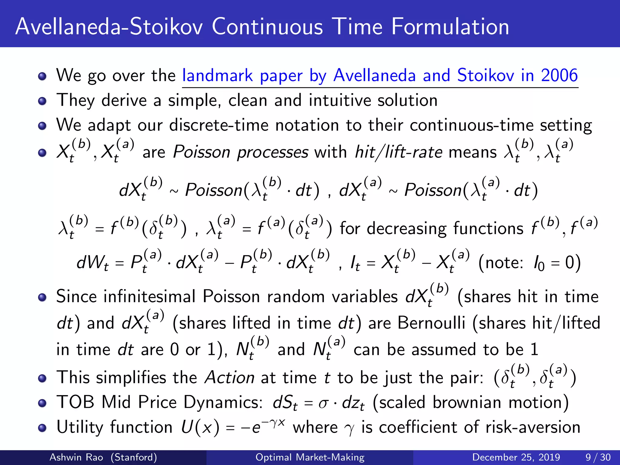
Notation for Optimal Market-Making Problem
We simplify the setting for ease of exposition
Assume ﬁnite time steps indexed by t = 0,1,...,T
Denote Wt ∈ R as Market-maker’s trading PnL at time t
Denote It ∈ Z as Market-maker’s inventory of shares at time t (I0 = 0)
St ∈ R+
is the TOB Mid Price at time t (assume stochastic process)
P
(b)
t ∈ R+
,N
(b)
t ∈ Z+
are market maker’s Bid Price, Bid Size at time t
P
(a)
t ∈ R+
,N
(a)
t ∈ Z+
are market-maker’s Ask Price, Ask Size at time t
Assume market-maker can add or remove bids/asks costlessly
Denote δ
(b)
t = St − P
(b)
t as Bid Spread, δ
(a)
t = P
(a)
t − St as Ask Spread
Random var X
(b)
t ∈ Z≥0 denotes bid-shares “hit” up to time t
Random var X
(a)
t ∈ Z≥0 denotes ask-shares “lifted” up to time t
Wt+1 = Wt +P
(a)
t ⋅(X
(a)
t+1 −X
(a)
t )−P
(b)
t ⋅(X
(b)
t+1 −X
(b)
t ) , It = X
(b)
t −X
(a)
t
Goal to maximize E[U(WT + IT ⋅ ST )] for appropriate concave U(⋅)

Markov Decision Process (MDP) Formulation
Order of MDP activity in each time step 0 ≤ t ≤ T − 1:
Observe State = (t,St,Wt,It)
Perform Action = (P
(b)
t ,N
(b)
t ,P
(a)
t ,N
(a)
t )
Experience TOB Dynamics resulting in:
random bid-shares hit = X
(b)
t+1 − X
(b)
t and ask-shares lifted = X
(a)
t+1 − X
(a)
t
update of Wt to Wt+1, update of It to It+1
stochastic evolution of St to St+1
Receive next-step (t + 1) Reward Rt+1
Rt+1 =
⎧⎪⎪
⎨
⎪⎪⎩
0 for 1 ≤ t + 1 ≤ T − 1
U(Wt+1 + It+1 ⋅ St+1) for t + 1 = T
Goal is to ﬁnd an Optimal Policy π∗
:
π∗
(t,St,Wt,It) = (P
(b)
t ,N
(b)
t ,P
(a)
t ,N
(a)
t ) that maximizes E[
T
∑
t=1
Rt]
Note: Discount Factor when aggregating Rewards in the MDP is 1

Avellaneda-Stoikov Continuous Time Formulation
We go over the landmark paper by Avellaneda and Stoikov in 2006
They derive a simple, clean and intuitive solution
We adapt our discrete-time notation to their continuous-time setting
X
(b)
t ,X
(a)
t are Poisson processes with hit/lift-rate means λ
(b)
t ,λ
(a)
t
dX
(b)
t ∼ Poisson(λ
(b)
t ⋅ dt) , dX
(a)
t ∼ Poisson(λ
(a)
t ⋅ dt)
λ
(b)
t = f (b)
(δ
(b)
t ) , λ
(a)
t = f (a)
(δ
(a)
t ) for decreasing functions f (b)
,f (a)
dWt = P
(a)
t ⋅ dX
(a)
t − P
(b)
t ⋅ dX
(b)
t , It = X
(b)
t − X
(a)
t (note: I0 = 0)
Since infinitesimal Poisson random variables dX
(b)
t (shares hit in time
dt) and dX
(a)
t (shares lifted in time dt) are Bernoulli (shares hit/lifted
in time dt are 0 or 1), N
(b)
t and N
(a)
t can be assumed to be 1
This simplifies the Action at time t to be just the pair: (δ
(b)
t ,δ
(a)
t )
TOB Mid Price Dynamics: dSt = σ ⋅ dzt (scaled brownian motion)
Utility function U(x) = −e−γx
where γ is coefficient of risk-aversion

Hamilton-Jacobi-Bellman (HJB) Equation
We denote the Optimal Value function as V ∗
(t,St,Wt,It)
V ∗
(t,St,Wt,It) = max
δ
(b)
t ,δ
(a)
t
E[−e−γ⋅(WT +It ⋅ST )
]
V ∗
(t,St,Wt,It) satisﬁes a recursive formulation for 0 ≤ t < t1 < T:
V ∗
(t,St,Wt,It) = max
δ
(b)
t ,δ
(a)
t
E[V ∗
(t1,St1 ,Wt1 ,It1 )]
Rewriting in stochastic diﬀerential form, we have the HJB Equation
max
δ
(b)
t ,δ
(a)
t
E[dV ∗
(t,St,Wt,It)] = 0 for t < T
V ∗
(T,ST ,WT ,IT ) = −e−γ⋅(WT +IT ⋅ST )

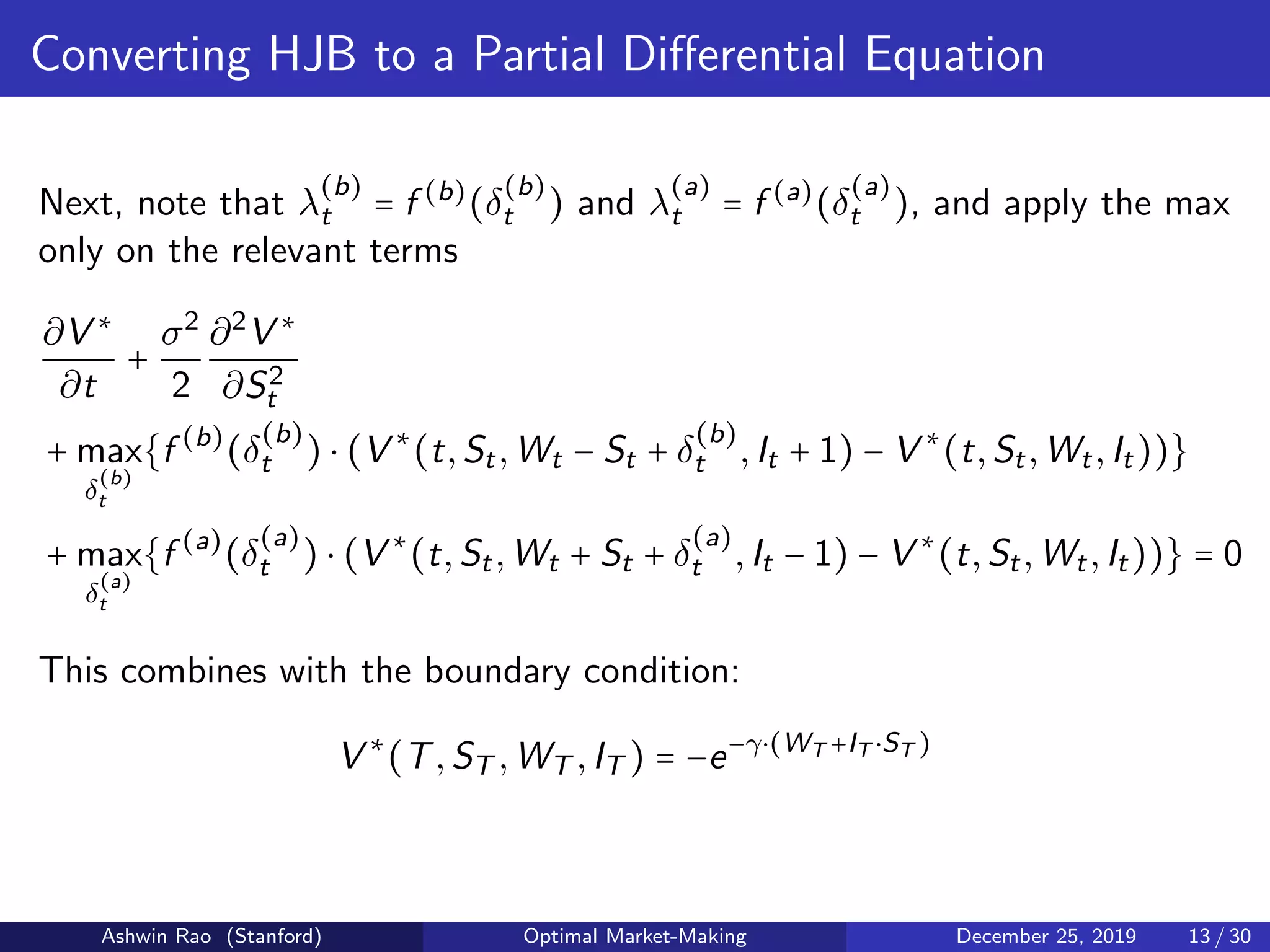
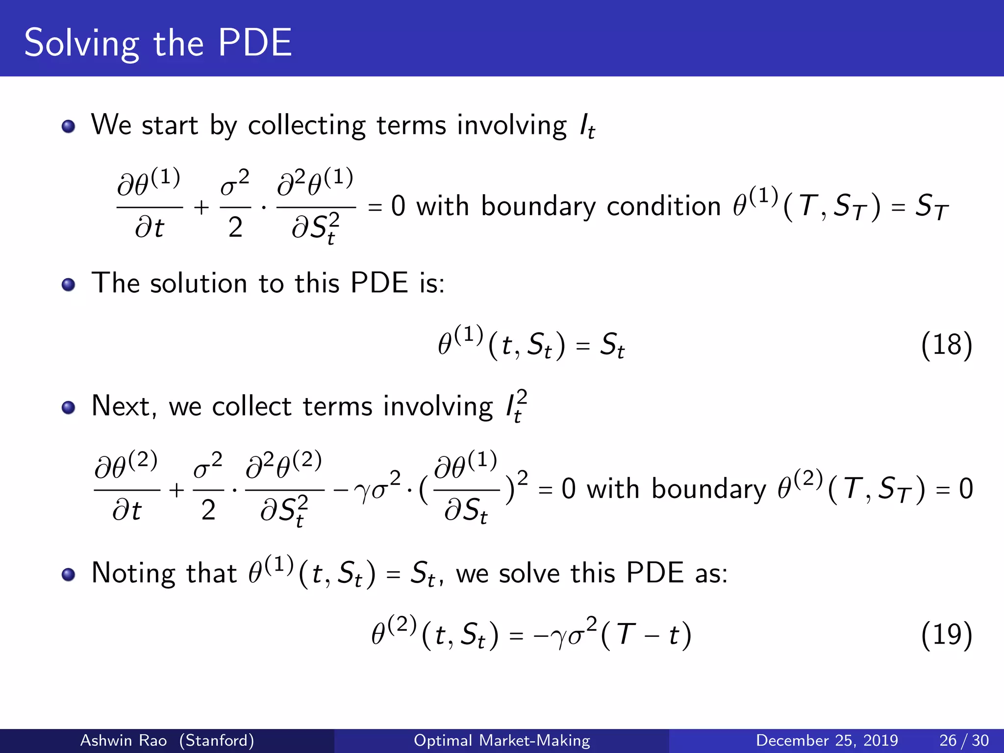
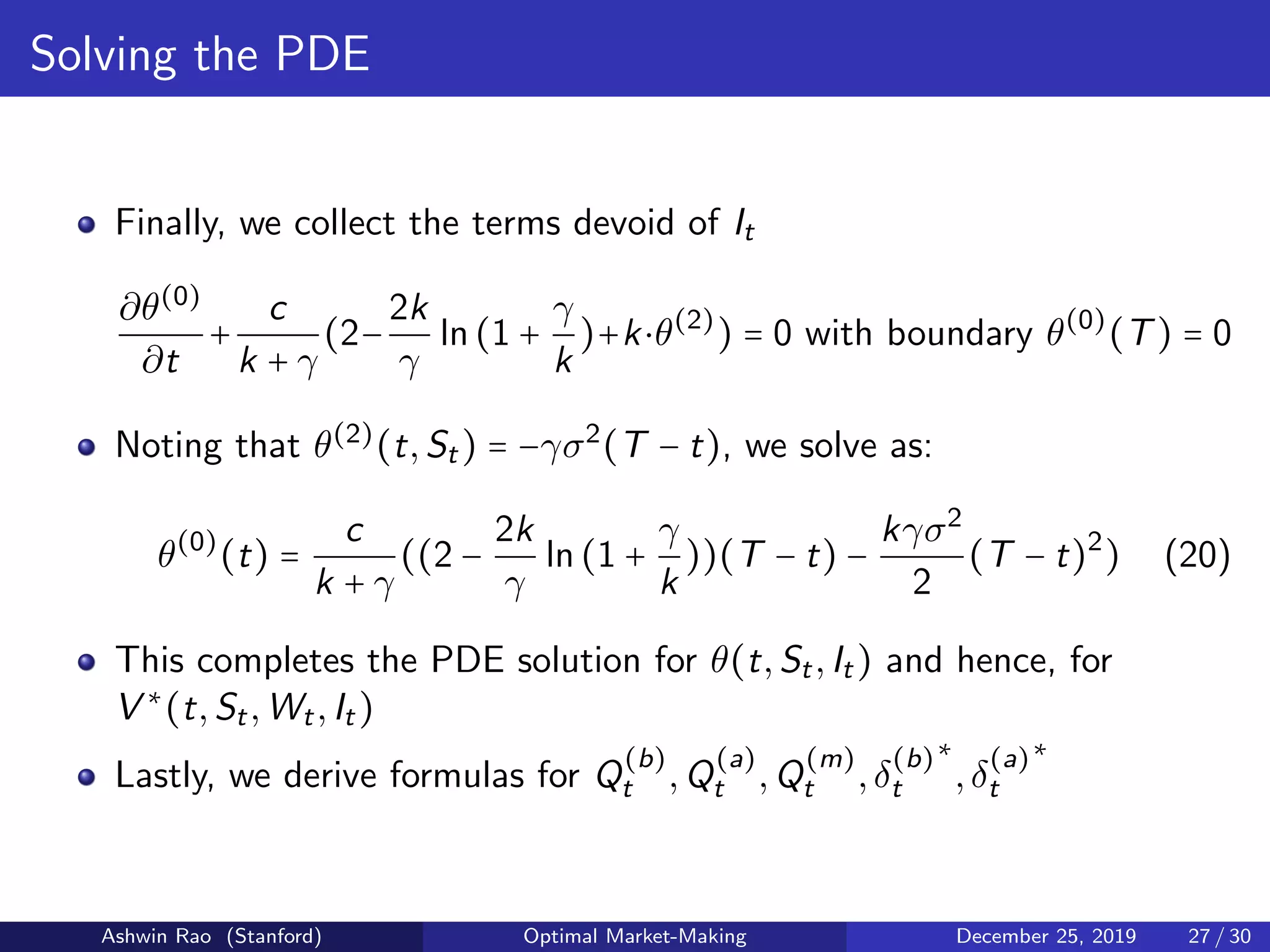
Converting HJB to a Partial Diﬀerential Equation
Change to V ∗
(t,St,Wt,It) is comprised of 3 components:
Due to pure movement in time t
Due to randomness in TOB Mid-Price St
Due to randomness in hitting/lifting the Bid/Ask
With this, we can expand dV ∗
(t,St,Wt,It) and rewrite HJB as:
max
δ
(b)
t ,δ
(a)
t
{
∂V ∗
∂t
dt + E[σ
∂V ∗
∂St
dzt +
σ2
2
∂2
V ∗
∂S2
t
(dzt)2
]
+ λ
(b)
t ⋅ dt ⋅ V ∗
(t,St,Wt − St + δ
(b)
t ,It + 1)
+ λ
(a)
t ⋅ dt ⋅ V ∗
(t,St,Wt + St + δ
(a)
t ,It − 1)
+ (1 − λ
(b)
t ⋅ dt − λ
(a)
t ⋅ dt) ⋅ V ∗
(t,St,Wt,It)
− V ∗
(t,St,Wt,It)} = 0

We can simplify this equation with a few observations:
E[dzt] = 0
E[(dzt)2
] = dt
Organize the terms involving λ
(b)
t and λ
(a)
t better with some algebra
Divide throughout by dt
max
δ
(b)
t ,δ
(a)
t
{
∂V ∗
∂t
+
σ2
2
∂2
V ∗
∂S2
t
+ λ
(b)
t ⋅ (V ∗
(b)
t ,It + 1) − V ∗
(t,St,Wt,It))
+ λ
(a)
t ⋅ (V ∗
(t,St,Wt + St + δ
(a)
t ,It − 1) − V ∗
(t,St,Wt,It))} = 0

Next, note that λ
(b)
t = f (b)
(δ
(b)
t ) and λ
(a)
t = f (a)
(δ
(a)
t ), and apply the max
only on the relevant terms
∂V ∗
∂t
+
σ2
2
∂2
V ∗
∂S2
t
+ max
δ
(b)
t
{f (b)
(δ
(b)
t ) ⋅ (V ∗
(b)
t ,It + 1) − V ∗
(t,St,Wt,It))}
+ max
δ
(a)
t
{f (a)
(δ
(a)
t ) ⋅ (V ∗
(t,St,Wt + St + δ
(a)
t ,It − 1) − V ∗
(t,St,Wt,It))} = 0
This combines with the boundary condition:
V ∗
(T,ST ,WT ,IT ) = −e−γ⋅(WT +IT ⋅ST )

We make an “educated guess” for the structure of V ∗
(t,St,Wt,It):
V ∗
(t,St,Wt,It) = −e−γ(Wt +θ(t,St ,It ))
(1)
and reduce the problem to a PDE in terms of θ(t,St,It)
Substituting this into the above PDE for V ∗
(t,St,Wt,It) gives:
∂θ
∂t
+
σ2
2
(
∂2
θ
∂S2
t
− γ(
∂θ
∂St
)2
)
+ max
δ
(b)
t
{
f (b)
(δ
(b)
t )
γ
⋅ (1 − e−γ(δ
(b)
t −St +θ(t,St ,It +1)−θ(t,St ,It ))
)}
+ max
δ
(a)
t
{
f (a)
(δ
(a)
t )
γ
⋅ (1 − e−γ(δ
(a)
t +St +θ(t,St ,It −1)−θ(t,St ,It ))
)} = 0
The boundary condition is:
θ(T,ST ,IT ) = IT ⋅ ST

Indifference Bid/Ask Price
It turns out that θ(t,St,It + 1) − θ(t,St,It) and
θ(t,St,It) − θ(t,St,It − 1) are equal to financially meaningful
quantities known as Indifference Bid and Ask Prices
Indifference Bid Price Q(b)
(t,St,It) is defined as:
V ∗
(t,St,Wt − Q(b)
(t,St,It),It + 1) = V ∗
(t,St,Wt,It) (2)
Q(b)
(t,St,It) is the price to buy a share with guarantee of immediate
purchase that results in Optimum Expected Utility being unchanged
Likewise, Indifference Ask Price Q(a)
(t,St,It) is defined as:
V ∗
(t,St,Wt + Q(a)
(t,St,It),It − 1) = V ∗
(t,St,Wt,It) (3)
Q(a)
(t,St,It) is the price to sell a share with guarantee of immediate
sale that results in Optimum Expected Utility being unchanged
We abbreviate Q(b)
(t,St,It) as Q
(b)
t and Q(a)
(t,St,It) as Q
(a)
t

Indiﬀerence Bid/Ask Price in the PDE for θ
Express V ∗
(t,St,Wt − Q
(b)
t ,It + 1) = V ∗
(t,St,Wt,It) in terms of θ:
−e−γ(Wt −Q
(b)
t +θ(t,St ,It +1))
= −e−γ(Wt +θ(t,St ,It ))
⇒ Q
(b)
t = θ(t,St,It + 1) − θ(t,St,It) (4)
Likewise for Q
(a)
t , we get:
Q
(a)
t = θ(t,St,It) − θ(t,St,It − 1) (5)
Using equations (4) and (5), bring Q
(b)
t and Q
(a)
t in the PDE for θ
∂θ
∂t
+
σ2
2
(
∂2
θ
∂S2
t
− γ(
∂θ
∂St
)2
) + max
δ
(b)
t
g(δ
(b)
t ) + max
δ
(a)
t
h(δ
(b)
t ) = 0
where g(δ
(b)
t ) =
f (b)
(δ
(b)
t )
γ
⋅ (1 − e−γ(δ
(b)
t −St +Q
(b)
t )
)
and h(δ
(a)
t ) =
f (a)
(δ
(a)
t )
γ
⋅ (1 − e−γ(δ
(a)
t +St −Q
(a)
t )
)

Optimal Bid Spread and Optimal Ask Spread
To maximize g(δ
(b)
t ), diﬀerentiate g with respect to δ
(b)
t and set to 0
e−γ(δ
(b)
t
∗
−St +Q
(b)
t )
⋅ (γ ⋅ f (b)
(δ
(b)
t
∗
) −
∂f (b)
∂δ
(b)
t
(δ
(b)
t
∗
)) +
∂f (b)
∂δ
(b)
t
(δ
(b)
t
∗
) = 0
⇒ δ
(b)
t
∗
= St − Q
(b)
t +
1
γ
⋅ ln(1 − γ ⋅
f (b)
(δ
(b)
t
∗
)
∂f (b)
∂δ
(b)
t
(δ
(b)
t
∗
)
) (6)
To maximize g(δ
(a)
t ), diﬀerentiate g with respect to δ
(a)
t and set to 0
e−γ(δ
(a)
t
∗
+St −Q
(a)
t )
⋅ (γ ⋅ f (a)
(δ
(a)
t
∗
) −
∂f (a)
∂δ
(a)
t
(δ
(a)
t
∗
)) +
∂f (a)
∂δ
(a)
t
(δ
(a)
t
∗
) = 0
⇒ δ
(a)
t
∗
= Q
(a)
t − St +
1
γ
⋅ ln(1 − γ ⋅
f (a)
(δ
(a)
t
∗
)
∂f (a)
∂δ
(a)
t
(δ
(a)
t
∗
)
) (7)
(6) and (7) are implicit equations for δ
(b)
t
∗
and δ
(a)
t
∗
respectively

Solving for θ and for Optimal Bid/Ask Spreads
Let us write the PDE in terms of the Optimal Bid and Ask Spreads
∂θ
∂t
+
σ2
2
(
∂2
θ
∂S2
t
− γ(
∂θ
∂St
)2
)
+
f (b)
(δ
(b)
t
∗
)
γ
⋅ (1 − e−γ(δ
(b)
t
∗
−St +θ(t,St ,It +1)−θ(t,St ,It ))
)
+
f (a)
(δ
(a)
t
∗
)
γ
⋅ (1 − e−γ(δ
(a)
t
∗
+St +θ(t,St ,It −1)−θ(t,St ,It ))
) = 0
with boundary condition θ(T,ST ,IT ) = IT ⋅ ST
(8)
First we solve PDE (8) for θ in terms of δ
(b)
t
∗
and δ
(a)
t
∗
In general, this would be a numerical PDE solution
Using (4) and (5), we have Q
(b)
t and Q
(a)
t in terms of δ
(b)
t
∗
and δ
(a)
t
∗
Substitute above-obtained Q
(b)
t and Q
(a)
t in equations (6) and (7)
Solve implicit equations for δ
(b)
t
∗
and δ
(a)
t
∗
(in general, numerically)

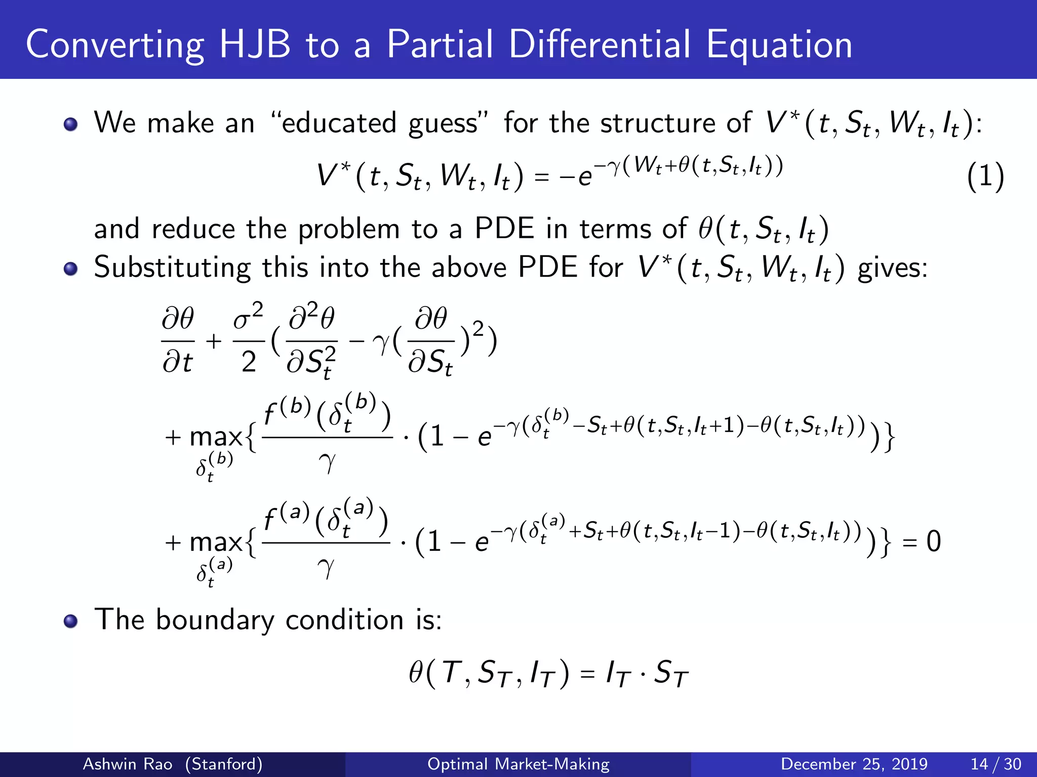
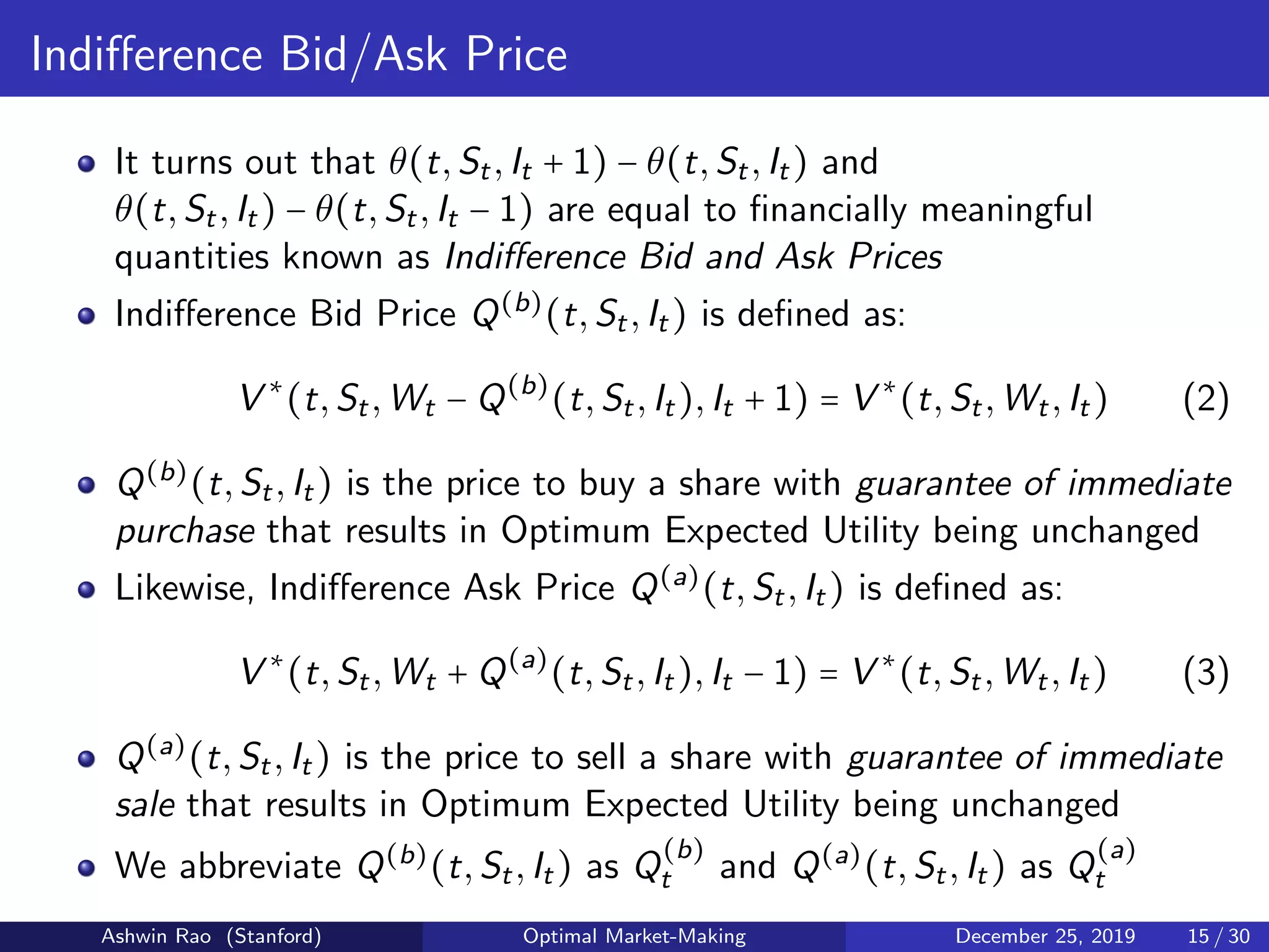
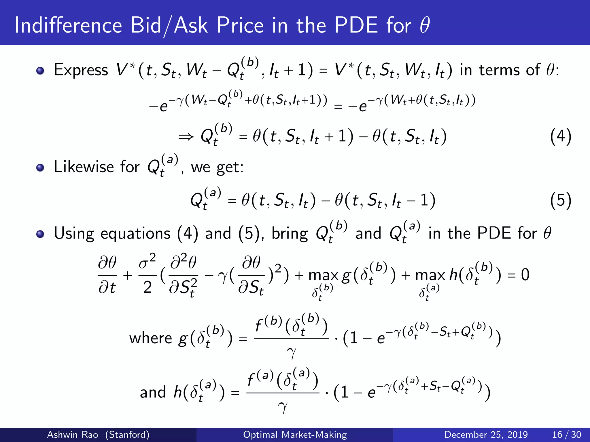
Building Intuition
Define Indifference Mid Price Q
(m)
t =
Q
(b)
t +Q
(a)
t
2
To develop intuition for Indifference Prices, consider a simple case
where the market-maker doesn’t supply any bids or asks
V ∗
(t,St,Wt,It) = E[−e−γ(Wt +It ⋅ST )
]
Combining this with the diffusion dSt = σ ⋅ dzt, we get:
V ∗
(t,St,Wt,It) = −e−γ(Wt +It ⋅St −
γ⋅I2
t ⋅σ2(T−t)
2
)
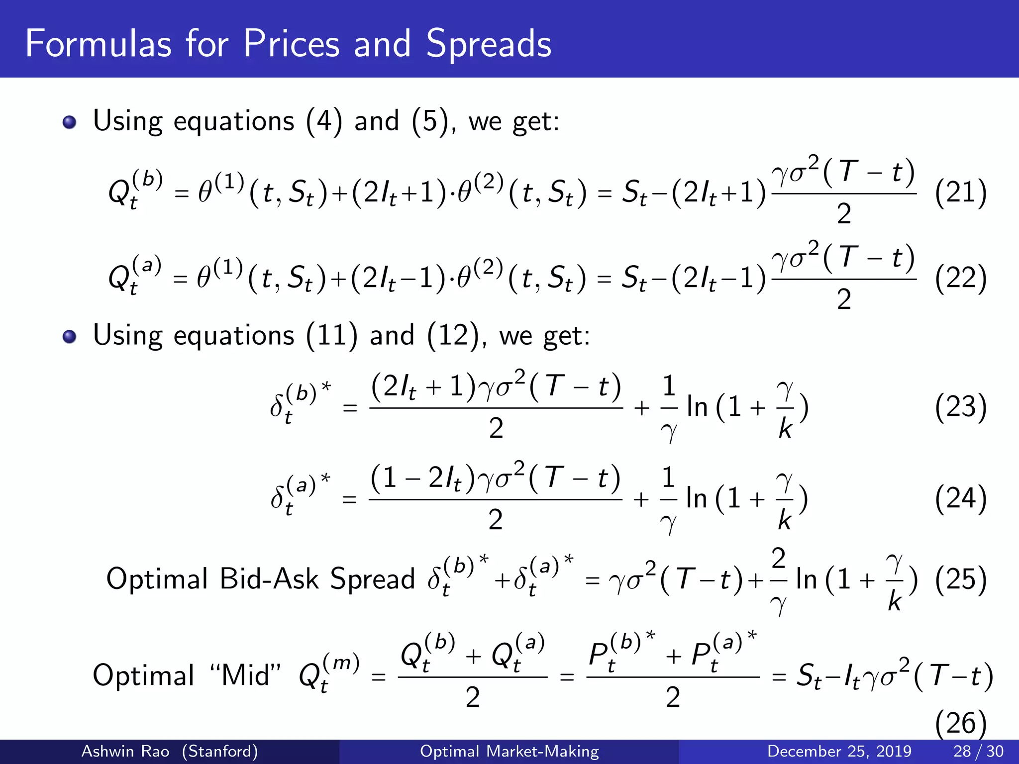
Combining this with equations (2) and (3), we get:
Q
(b)
t = St − (2It + 1)
γσ2
(T − t)
2
, Q
(a)
t = St − (2It − 1)
γσ2
(T − t)
2
Q
(m)
t = St − Itγσ2
(T − t) , Q
(a)
t − Q
(b)
t = γσ2
(T − t)
These results for the simple case of no-market-making serve as
approximations for our problem of optimal market-making

Building Intuition
Think of Q
(m)
t as inventory-risk-adjusted mid-price (adjustment to St)
If market-maker is long inventory (It > 0), Q
(m)
t < St indicating
inclination to sell than buy, and if market-maker is short inventory,
Q
(m)
t > St indicating inclination to buy than sell
Armed with this intuition, we come back to optimal market-making,
observing from eqns (6) and (7): P
(b)
t
∗
< Q
(b)
t < Q
(m)
t < Q
(a)
t < P
(a)
t
∗
Think of [P
(b)
t
∗
,P
(a)
t
∗
] as “centered” at Q
(m)
t (rather than at St),
i.e., [P
(b)
t
∗
,P
(a)
t
∗
] will (together) move up/down in tandem with
Q
(m)
t moving up/down (as a function of inventory position It)
Q
(m)
t − P
(b)
t
∗
=
Q
(a)
t − Q
(b)
t
2
+
1
γ
⋅ ln(1 − γ ⋅
f (b)
(δ
(b)
t
∗
)
∂f (b)
∂δ
(b)
t
(δ
(b)
t
∗
)
) (9)
P
(a)
t
∗
− Q
(m)
t =
Q
(a)
t − Q
(b)
t
2
+
1
γ
⋅ ln(1 − γ ⋅
f (a)
(δ
(a)
t
∗
)
∂f (a)
∂δ
(a)
t
(δ
(a)
t
∗
)
) (10)

Simple Functional Form for Hitting/Lifting Rate Means
The PDE for θ and the implicit equations for δ
(b)
t
∗
,δ
(a)
t
∗
are messy
We make some assumptions, simplify, derive analytical approximations
First we assume a fairly standard functional form for f (b)
and f (a)
f (b)
(δ) = f (a)
(δ) = c ⋅ e−k⋅δ
This reduces equations (6) and (7) to:
δ
(b)
t
∗
= St − Q
(b)
t +
1
γ
ln(1 +
γ
k
) (11)
δ
(a)
t
∗
= Q
(a)
t − St +
1
γ
ln(1 +
γ
k
) (12)
⇒ P
(b)
t
∗
and P
(a)
t
∗
are equidistant from Q
(m)
t
Substituting these simpliﬁed δ
(b)
t
∗
,δ
(a)
t
∗
in (8) reduces the PDE to:
∂θ
∂t
+
σ2
2
(
∂2
θ
∂S2
t
− γ(
∂θ
∂St
)2
) +
c
k + γ
(e−k⋅δ
(b)
t
∗
+ e−k⋅δ
(a)
t
∗
) = 0
with boundary condition θ(T,ST ,IT ) = IT ⋅ ST
(13)

Simplifying the PDE with Approximations
Note that this PDE (13) involves δ
(b)
t
∗
and δ
(a)
t
∗
However, equations (11), (12), (4), (5) enable expressing δ
(b)
t
∗
and
δ
(a)
t
∗
in terms of θ(t,St,It − 1),θ(t,St,It),θ(t,St,It + 1)
This would give us a PDE just in terms of θ
Solving that PDE for θ would not only give us V ∗
(t,St,Wt,It) but
also δ
(b)
t
∗
and δ
(a)
t
∗
(using equations (11), (12), (4), (5) )
To solve the PDE, we need to make a couple of approximations
First we make a linear approx for e−k⋅δ
(b)
t
∗
and e−k⋅δ
(a)
t
∗
in PDE (13):
∂θ
∂t
+
σ2
2
(
∂2
θ
∂S2
t
− γ(
∂θ
∂St
)2
) +
c
k + γ
(1 − k ⋅ δ
(b)
t
∗
+ 1 − k ⋅ δ
(a)
t
∗
) = 0 (14)
Equations (11), (12), (4), (5) tell us that:
δ
(b)
t
∗
+δ
(a)
t
∗
=
2
γ
ln(1 +
γ
k
)+2θ(t,St,It)−θ(t,St,It +1)−θ(t,St,It −1)

Asymptotic Expansion of θ in It
With this expression for δ
(b)
t
∗
+ δ
(a)
t
∗
, PDE (14) takes the form:
∂θ
∂t
+
σ2
2
(
∂2
θ
∂S2
t
− γ(
∂θ
∂St
)2
) +
c
k + γ
(2 −
2k
γ
ln(1 +
γ
k
)
− k(2θ(t,St,It) − θ(t,St,It + 1) − θ(t,St,It − 1))) = 0
(15)
To solve PDE (15), we consider this asymptotic expansion of θ in It:
θ(t,St,It) =
∞
∑
n=0
In
t
n!
⋅ θ(n)
(t,St)
So we need to determine the functions θ(n)
(t,St) for all n = 0,1,2,...
For tractability, we approximate this expansion to the ﬁrst 3 terms:
θ(t,St,It) ≈ θ(0)
(t,St) + It ⋅ θ(1)
(t,St) +
I2
t
2
⋅ θ(2)
(t,St)

Approximation of the Expansion of θ in It
We note that the Optimal Value Function V ∗
can depend on St only
through the current Value of the Inventory (i.e., through It ⋅ St), i.e.,
it cannot depend on St in any other way
This means V ∗
(t,St,Wt,0) = −e−γ(Wt +θ(0)(t,St ))
is independent of St
This means θ(0)
(t,St) is independent of St
So, we can write it as simply θ(0)
(t), meaning ∂θ(0)
∂St
and ∂2θ(0)
∂S2
t
are 0
Therefore, we can write the approximate expansion for θ(t,St,It) as:
θ(t,St,It) = θ(0)
(t) + It ⋅ θ(1)
(t,St) +
I2
t
2
⋅ θ(2)
(t,St) (16)

Solving the PDE
Substitute this approximation (16) for θ(t,St,It) in PDE (15)
∂θ(0)
∂t
+ It
∂θ(1)
∂t
+
I2
t
2
∂θ(2)
∂t
+
σ2
2
(It
∂2
θ(1)
∂S2
t
+
I2
t
2
∂2
θ(2)
∂S2
t
)
−
γσ2
2
(It
∂θ(1)
∂St
+
I2
t
2
∂θ(2)
∂St
)2
+
c
k + γ
(2 −
2k
γ
ln(1 +
γ
k
) + k ⋅ θ(2)
) = 0
with boundary condition:
θ(0)
(T) + IT ⋅ θ(1)
(T,ST ) +
I2
T
2
⋅ θ(2)
(T,ST ) = IT ⋅ ST
(17)
We will separately collect terms involving speciﬁc powers of It, each
yielding a separate PDE:
Terms devoid of It (i.e., I0
t )
Terms involving It (i.e., I1
t )
Terms involving I2
t

Solving the PDE
We start by collecting terms involving It
∂θ(1)
∂t
+
σ2
2
⋅
∂2
θ(1)
∂S2
t
= 0 with boundary condition θ(1)
(T,ST ) = ST
The solution to this PDE is:
θ(1)
(t,St) = St (18)
Next, we collect terms involving I2
t
∂θ(2)
∂t
+
σ2
2
⋅
∂2
θ(2)
∂S2
t
−γσ2
⋅(
∂θ(1)
∂St
)2
= 0 with boundary θ(2)
(T,ST ) = 0
Noting that θ(1)
(t,St) = St, we solve this PDE as:
θ(2)
(t,St) = −γσ2
(T − t) (19)

Solving the PDE
Finally, we collect the terms devoid of It
∂θ(0)
∂t
+
c
k + γ
(2−
2k
γ
ln(1 +
γ
k
)+k⋅θ(2)
) = 0 with boundary θ(0)
(T) = 0
Noting that θ(2)
(t,St) = −γσ2
(T − t), we solve as:
θ(0)
(t) =
c
k + γ
((2 −
2k
γ
ln(1 +
γ
k
))(T − t) −
kγσ2
2
(T − t)2
) (20)
This completes the PDE solution for θ(t,St,It) and hence, for
V ∗
(t,St,Wt,It)
Lastly, we derive formulas for Q
(b)
t ,Q
(a)
t ,Q
(m)
t ,δ
(b)
t
∗
,δ
(a)
t
∗

Formulas for Prices and Spreads
Using equations (4) and (5), we get:
Q
(b)
t = θ(1)
(t,St)+(2It +1)⋅θ(2)
(t,St) = St −(2It +1)
γσ2
(T − t)
2
(21)
Q
(a)
t = θ(1)
(t,St)+(2It −1)⋅θ(2)
(t,St) = St −(2It −1)
γσ2
(T − t)
2
(22)
Using equations (11) and (12), we get:
δ
(b)
t
∗
=
(2It + 1)γσ2
(T − t)
2
+
1
γ
ln(1 +
γ
k
) (23)
δ
(a)
t
∗
=
(1 − 2It)γσ2
(T − t)
2
+
1
γ
ln(1 +
γ
k
) (24)
Optimal Bid-Ask Spread δ
(b)
t
∗
+δ
(a)
t
∗
= γσ2
(T −t)+
2
γ
ln(1 +
γ
k
) (25)
Optimal “Mid” Q
(m)
t =
Q
(b)
t + Q
(a)
t
2
=
P
(b)
t
∗
+ P
(a)
t
∗
2
= St−Itγσ2
(T−t)
(26)

Back to Intuition
Think of Q
(m)
t as inventory-risk-adjusted mid-price (adjustment to St)
If market-maker is long inventory (It > 0), Q
(m)
t < St indicating
inclination to sell than buy, and if market-maker is short inventory,
Q
(m)
t > St indicating inclination to buy than sell
Think of [P
(b)
t
∗
,P
(a)
t
∗
] as “centered” at Q
(m)
t (rather than at St),
i.e., [P
(b)
t
∗
,P
(a)
t
∗
] will (together) move up/down in tandem with
Q
(m)
t moving up/down (as a function of inventory position It)
Note from equation (25) that the Optimal Bid-Ask Spread
P
(a)
t
∗
− P
(b)
t
∗
is independent of inventory It
Useful view: P
(b)
t
∗
< Q
(b)
t < Q
(m)
t < Q
(a)
t < P
(a)
t
∗
, with these spreads:
Outer Spreads P
(a)
t
∗
− Q
(a)
t = Q
(b)
t − P
(b)
t
∗
=
1
γ
ln(1 +
γ
k
)
Inner Spreads Q
(a)
t − Q
(m)
t = Q
(m)
t − Q
(b)
t =
γσ2
(T − t)
2

Real-world Market-Making and Reinforcement Learning
Real-world TOB dynamics are non-stationary, non-linear, complex
Frictions: Discrete Prices/Sizes, Constraints on Prices/Sizes, Fees
Need to capture various market factors in the State & TOB Dynamics
This leads to Curse of Dimensionality and Curse of Modeling
The practical route is to develop a simulator capturing all of the above
Simulator is a Market-Data-learnt Sampling Model of TOB Dynamics
Using this simulator and neural-networks func approx, we can do RL
References: 2018 Paper from University of Liverpool and
2019 Paper from JP Morgan Research
Exciting area for Future Research as well as Engineering Design

Stochastic Control/Reinforcement Learning for Optimal Market Making

More Related Content

Similar to Stochastic Control/Reinforcement Learning for Optimal Market Making

More from Ashwin Rao

Recently uploaded

Stochastic Control/Reinforcement Learning for Optimal Market Making