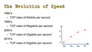
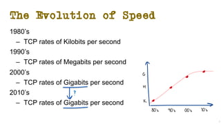
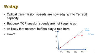
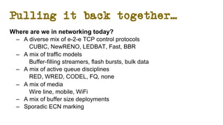
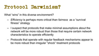
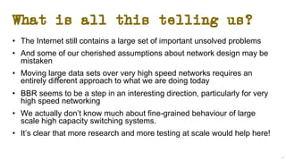
The document discusses the evolution of Transmission Control Protocol (TCP) speeds and the impact of network buffers on these speeds, highlighting the historical progression from kilobits to terabits while detailing TCP's flow control mechanisms. It explains various TCP algorithms, such as Reno and Cubic, and their adaptations to manage buffer sizes and improve network efficiency. The document emphasizes current challenges in networking and stresses the need for further research to address unsolved issues and enhance high-speed data transmission.

1. Buffers and Protocols
Geoff Huston
APNIC Labs

2. The Evolution of Speed
1980’s
– TCP rates of Kilobits per second
1990’s
– TCP rates of Megabits per second
2000’s
– TCP rates of Gigabits per second
2010’s
– TCP rates of Gigabits per second
2
80’s 90’s 00’s 10’s
K
M
G

3. The Evolution of Speed
1980’s
– TCP rates of Kilobits per second
1990’s
– TCP rates of Megabits per second
2000’s
– TCP rates of Gigabits per second
2010’s
– TCP rates of Gigabits per second
3
80’s 90’s 00’s 10’s
K
M
G
?

4. Today
• Optical transmission speeds are now edging into Terrabit
capacity
• But peak TCP session speeds are not keeping up
• Its likely that network buffers play a role here
• How?
480’s 90’s 00’s 10’s
K
M
G
T
optical
transport
TCP speed

5. TCP
• The Transmission Control Protocol is an end-to-end
protocol that creates a reliable stream protocol from the
underlying IP datagram device
• TCP operates as an adaptive rate control protocol that
attempts to operate efficiently and fairly

6. TCP Design Objectives
To maintain an average flow which is Efficient and Fair
Efficient:
– Minimise packet loss
– Minimise packet re-ordering
– Do not leave unused path bandwidth on the table!
Fair:
– Do not crowd out other TCP sessions
– Over time, take an average 1/N of the path capacity when there are
N other TCP sessions sharing the same path

7. It’s a Flow Control process
• Think of this as a multi-
flow fluid dynamics
problem
• Each flow has to gently
exert pressure on the
other flows to signal
them to provide a fair
share of the network,
and be responsive to
the pressure from all
other flows

8. TCP Control
TCP is an ACK Pacing protocol
Data sending rate is matched to the
ACK arrival rate

9. TCP Control
• Ideally TCP would send packets at a fair share of
available network capacity. But the TCP sender has no
idea what “available network capacity” means.
• So TCP uses ‘rate adaptation’ to probe into network,
increasing the sending rate until it is ‘too fast’
• Packet drop is the conventional signal of ‘too fast”

10. TCP Control
ACK pacing protocols relate to a past network state, not necessarily the
current network state
– The ACK signal shows the rate of data that left the network at the
receiver that occurred at ½ RTT back in time
– If there is data loss in the forward path, the ACK signal of that loss is
already at least ½ RTT old!
TCP should react quickly to ‘bad’ news
– If there is no data loss, that is also old news
TCP should react conservatively to ‘good’ news

11. “Classic TCP” – TCP Reno
• Additive Increase Multiplicative Decrease (AIMD)
– While there is no packet loss, increase the sending rate by one
segment (MSS) each RTT interval
– If there is packet loss decrease the sending rate by 50% over the
next RTT Interval, and halve the sender’s window
• Start Up
– Each RTT interval, double the sending rate
– We call this “slow start” – probably because its anything but slow!!!

12. TCP Reno and Buffers – the Theory
Queue formation
Queue drain

13. TCP and Buffers – the Theory
• When a sender receives a low signal it repairs the loss and
halves its sending window
• This will cause the sender to pause for the amount of time to
drain halve the outstanding data in the network
• Ideally this exactly matches the amount of time taken for the
queue to drain
• At the time the queue is drained the sender resumes its sending
(at half the rate) and the buffer has fully drained
• For this to work, the queue size should equal the delay
bandwidth product of the link it drives

14. TCP and Buffers – the Theory
• When a sender receives a low signal it repairs the loss and
halves its sending window
• This will cause the sender to pause for the amount of time to
drain halve the outstanding data in the network
• Ideally this exactly matches the amount of time taken for the
queue to drain
• At the time the queue is drained the sender resumes its sending
(at half the rate) and the buffer has fully drained
• For this to work, the queue size should equal the delay
bandwidth product of the link it drives
All this works with an assumption of a single queue and a single flow

15. TCP and Buffers
• The rule of thumb for buffer size is
Size = (BW ∙ RTT)
15
“High Performance TCP in ANSNET”
Villamizar & Song, 1994

16. TCP and Buffers
Too Big: The queue never drains, so the buffer adds delay to
the connection
Sender’s window recovery interval
(1xRTT)
Congestion
AvoidanceCongestion
Avoidance
Time
SendingRate/SenderWindow
Packet Loss
Queue too big
Link Capacity
Added
delay

17. TCP and Buffers
Too Small: The queue drains and the sender operates below
bottleneck speed – so the link is under-used
Sender’s window recovery interval
(1xRTT)
Congestion
AvoidanceCongestion
Avoidance
Time
SendingRate/SenderWindow
Packet Loss
Queue too small
Link Capacity
Idle
capacity

18. Refinements to RENO
• There have been many efforts to alter RENO’s flow control algorithm
• In a loss-based AIMD control system the essential parameters are the
manner of rate increase and the manner of loss-based decrease
– For example:
MulTCP behaves as it it were N simultaneous TCP sessions: i.e.
increase by N segments each RTT and rate drop by 1/N upon
packet loss
• What about varying the manner of rate increase away from AI?

19. Enter CUBIC
• CUBIC is designed to be useful for high speed sessions while still
being ‘fair’ to other sessions and also efficient even at lower speeds
• Rather than probe in a linear manner for the sending rate that triggers
packet loss, CUBIC uses a non-linear (cubic) search algorithm

20. CUBIC and Queue formation
Total Queue Capacity
(Onset of Packet Loss)
Link Capacity Capacity
(Onset of Queuing)
Network Buffers Fill
Network Buffers Drain

21. CUBIC assessment
• Can react quickly to available capacity in the network
• Tends to sit for extended periods in the phase of queue
formation
• Can react efficiently to long fat pipes and rapidly scale up
the sending rate
• Operates in a manner that tends to exacerbate ‘buffer bloat’
conditions

22. From 1 to N – Scaling Switching
22
• This finding of buffer size relates to a single flow through a
single bottleneck resource
• What happens to buffers with more flows and faster
transmission system?

23. Flow Mixing
• If 2 flows use a single buffer and they resonate precisely
then the buffer still needs to be delay-bandwidth size
• If they are precisely out of phase the common buffer
requirement is halved
23

24. Smaller Buffers?
• If 2 flows use a single buffer and they resonate precisely then the buffer still
needs to be delay-bandwidth size
• If they are precisely out of phase the common buffer requirement is halved
• What about the case of N de-synchronised flows?
Size = (BW ∙ RTT) / √N
Assuming that the component flows manage to achieve a fair outcome of
obtaining 1/N of the resource in a non-synchronised manner, then the peak
buffer resource is inversely proportionate to the square root of N
24
(“Sizing Router Buffers”, Appenzeller, McKeown, Keslassy, SIGCOM’04)

25. The Role of Buffers
• Buffers in a network serve two essential roles:
– smooth sender burstiness
– Multiplexing N inputs to 1 output

26. Sender Pacing
• Distribute cwnd data across the entire RTT interval
• Remove burst adaptation pressure on network buffers

27. Tiny Buffers?
• If all senders ‘paced’ their sending to avoid bursting, and
were sensitive to the formation of standing queues then we
would likely have a residual multiplexing requirement for
buffers where:
B >= O(log W)
where W is the average flow window size
27

28. Why is this important?
• Because memory speed is not scaling at the same rate as
transmission or switching
• Further capacity and speed improvements in the network
mandate reduced memory demands within the switch

29. Switching Chip Design TradeOffs
• On Chip memory is fast, but limited to between ~16M to ~64M
• A chip design can include an interface to external memory banks
but the memory interface/controller also takes up chip space and
the external memory is slower
• Between 20% to 60% of switch chip real estate is devoted to
memory / memory control
• Small memory buffers in switch design allows for larger switch
fabric implementations on the chip
29

30. Switch Design
30

31. Flow States
• There are three ‘states’ of flow management:
– Under-Utilised – where the flow rate is below the link capacity and no queues
form
– Over-Utilised – where the flow rate is greater that the link capacity and queues
form
– Saturated – where the queue is filled and packet loss occurs
• Loss-based control systems probe upward to the Saturated point, and back off
quickly to what they guess is the Under-Utilised state in order to the let the queues
drain
• But the optimal operational point for any flow is at the point of state change from
Under to Over-utilised, not at the Saturated point

32. RTT and Delivery Rate with Queuing
Under-Utilised Over-Utilised Saturated

33. How to detect the onset of
queuing?
• By getting the network say when queues are forming

34. ICMP Source Quench Redux!
• Switch generates an ICMP message (similar to ICMP PTB)
• ICMP payload allows sender to identify TCP session

35. ICMP Issues
• IMCP messages are unverified
– DOS attack vector
• ICMP messages are often filtered
– A sender cannot rely upon the message
• Anycast can add subtle complications here!

36. Explicit Congestion Notification

37. Explicit Congestion Notification
• Sparse signal (single bit)
• Both hosts and routers need to be ECN aware
• IP level marking requires end host protocol surgery at both
ends:
• Receivers need to reflect ECN bits
• Senders need to pass IP ECN up to the TCP session

38. ECN Issues
• It would be good if…
– everyone did it!
• But they don’t all do it, which means that hosts cannot rely
on ECN as the only means of congestion control
• What’s the value of partial adoption of ECN?

39. High Precision Congestion Control
• Eliminate all the guesswork out of the problem by having
each switch attach the time, local queue length and link
bandwidth to the IP packet!

40. How to detect the onset of
queuing?
• By getting the network say when queues are forming
OR
• By detecting the onset of queue-based delays in the
measured RTT

41. Flow Control Revisited
• Current flow control systems make small continual adjustments every
RTT interval and a massive adjustment at irregular intervals
– As the flow rate increases the CA adjustments of 1 segment per RTT
become too small
– Rate halving is a massive response
OR
• We could use a system that only made periodic adjustments every n
RTT intervals
– And set the adjustment to be proportionate to the current flow rate
41

42. BBR Design Principles
• Pace the sending packets to avoid the need for network buffer rate
adaptation
• Probe the path capacity only intermittently (every 8th RTT)
• Probe the path capacity by increasing the sending rate by 25% for
an RTT interval and then drop the rate to drain the queue:
– If the RTT of the probe interval equals the RTT of the previous
state then there is available path bandwidth that could be utilised
– If the RTT of the probe rises then the path is likely to be at the
onset of queuing and no further path bandwidth is available
• Do not alter the path bandwidth estimate in response to packet loss

43. Idealised BBR profile
sending rate
network queues

44. BBR Politeness?
• BBR will probably not constantly
pull back when simultaneous
loss-based protocols exert
pressure on the path’s queues
• BBR tries to make minimal
demands on the queue size, and
does not rely on a large dynamic
range of queue occupancy
during a flow

45. Pulling it back together…
Where are we in networking today?
– A diverse mix of e-2-e TCP control protocols
CUBIC, NewRENO, LEDBAT, Fast, BBR
– A mix of traffic models
Buffer-filling streamers, flash bursts, bulk data
– A mix of active queue disciplines
RED, WRED, CODEL, FQ, none
– A mix of media
Wire line, mobile, WiFi
– A mix of buffer size deployments
– Sporadic ECN marking

46. Protocol Darwinism?
What “wins” in this diverse environment?
– Efficiency is perhaps more critical than fairness as a “survival
fitness” strategy
– I suspect that protocols that make minimal assumptions about the
network will be more robust than those that require certain network
characteristics to operate efficiently
– Protocols that operate with regular feedback mechanisms appear to
be more robust than irregular “shock” treatment protocols

47. What is all this telling us?
• The Internet still contains a large set of important unsolved problems
• And some of our cherished assumptions about network design may be
mistaken
• Moving large data sets over very high speed networks requires an
entirely different approach to what we are doing today
• BBR seems to be a step in an interesting direction, particularly for very
high speed networking
• We actually don’t know much about fine-grained behaviour of large
scale high capacity switching systems.
• It’s clear that more research and more testing at scale would help here!
47

48. That’s it!
Questions?