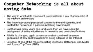
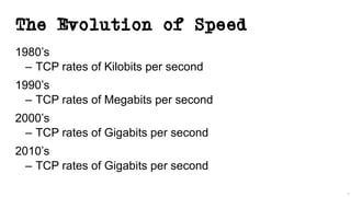
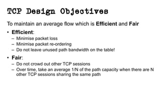
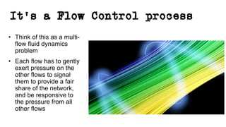
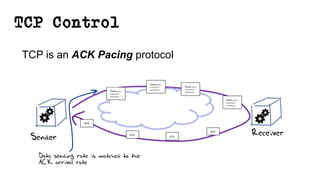
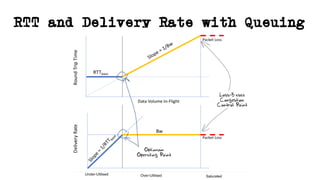
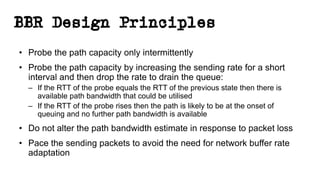
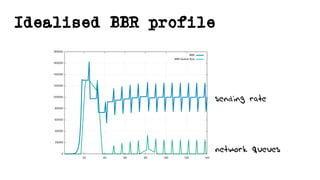
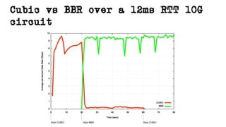
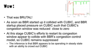
This document discusses TCP and a new flow control algorithm called BBR. It provides background on TCP and how its sending rate is controlled via ACK pacing. While TCP rates increased from kilobits to gigabits per second over time, it is not keeping up with optical transmission speeds approaching terabits. BBR aims to be more efficient than TCP by probing the network to detect the onset of queueing rather than relying on packet loss. Testing shows BBR can crowd out other flows and operate inefficiently against itself. While promising for high speeds, BBR may not scale well if widely adopted and requires further research to improve fairness against other flows.

1. TCP and BBR
Geoff Huston
APNIC

2. Computer Networking is all about
moving data
• The way in which data movement is controlled is a key characteristic of
the network architecture
• The Internet protocol passed all controls to the end systems, and
treated the network as a passive switching environment
• But that was many years ago, and since then we have seen the
deployment of active middleware in networks and control traffic flows
• All this is changing again as we see a what could well be a new
generation of flow control algorithms being adopted in the Internet
• Lets look at one of the more interesting initiatives: Bottleneck Bandwidth
and Round-Trip Time (BBR)
2

3. Let’s talk about speed
• How fast can we push a single session to move data
through the network?
• Session speed is the result of a combination of:
• available transmission speeds,
• end-to-end latency and
• protocol efficiency
– All of these factors are critical
3

4. The Evolution of Speed
1980’s
– TCP rates of Kilobits per second
1990’s
– TCP rates of Megabits per second
2000’s
– TCP rates of Gigabits per second
2010’s
– TCP rates of Gigabits per second
4

5. Today
• Optical transmission speeds are approaching Terrabit
capacity
• But peak TCP session speeds are not keeping up
• What’s going on?
5

6. TCP
• The Transmission Control Protocol is an end-to-end
protocol that creates a reliable stream protocol from the
underlying IP datagram device
• TCP operates as an adaptive rate control protocol that
attempts to operate fairly and efficiently

7. TCP Design Objectives
To maintain an average flow which is Efficient and Fair
• Efficient:
– Minimise packet loss
– Minimise packet re-ordering
– Do not leave unused path bandwidth on the table!
• Fair:
– Do not crowd out other TCP sessions
– Over time, take an average 1/N of the path capacity when there are N
other TCP sessions sharing the same path

8. It’s a Flow Control process
• Think of this as a multi-
flow fluid dynamics
problem
• Each flow has to gently
exert pressure on the
other flows to signal
them to provide a fair
share of the network,
and be responsive to
the pressure from all
other flows

9. TCP Control
TCP is an ACK Pacing protocol
Data sending rate is matched to the
ACK arrival rate

10. TCP Control
ACK pacing protocols relate to a past network state, not
necessarily the current network state
– The ACK signal shows the rate of data that left the network at the
receiver that occurred at ½ RTT back in time
– So if there is data loss, the ACK signal of that loss is already ½ RTT
old!
• So TCP should react quickly to ‘bad’ news
– If there is no data loss, that is also old news
• So TCP should react conservatively to ‘good’ news

11. “Classic TCP” – TCP Reno
• Additive Increase Multiplicative Decrease (AIMD)
– While there is no packet loss, increase the sending rate by One
Segment (MSS) each RTT interval
– If there is packet loss decrease the sending rate by 50% over the
next RTT Interval
• Start Up
– Each RTT interval, double the sending rate
– We call this “slow start” – probably because its anything but slow!!!

12. Idealised TCP Reno
Time
Slow Start
Rate Doubles
each RTT
Interval
Congestion Avoidance
Rate increases by 1 MSS per RTT
Rate halves on Packet Loss
Notification of Packet Loss
via Duplicate ACKs causes
RENO to halve its sending
rate

13. TCP RENO and Idealized Queue
Behaviour
Total Queue Capacity
(Onset of Packet Loss)
Link Capacity Capacity
(Onset of Queuing)
Network Buffers Fill
Network Buffers Drain

14. Reno is too slow
• TCP Reno tries to oscillate between sending rates R and 2 x R
that span the actual link capacity
• It increases its sending rate slowly so it’s really lousy when trying
to run at very high speed over long delay networks
• It over-corrects on loss and leaves available path capacity idle
– 10Gbps rates over 100ms RTT demands a packet loss rate of less than
0.000003%
– An average 1% loss rate over a 100ms RTT can’t operate faster than
3Mbps

15. Faster than Reno?
• Can we make TCP faster and more efficient by changing
the way in which the sending rate is inflated?
• Of course!

16. Refinements to RENO
• There have been many efforts to alter RENO’s flow control
algorithm
• In a loss-based AIMD control system the essential parameters
are the manner of rate increase and the manner of loss-based
decrease
– For example:
MulTCP behaves as it it were N simultaneous TCP sessions: i.e. increase by N segments
each RTT and rate drop by 1/N upon packet loss
• What about varying the manner of rate increase away from AI?

17. Enter CUBIC
• CUBIC is designed to be useful for high speed sessions while still
being ‘fair’ to other sessions and also efficient even at lower speeds
• Rather than probe in a linear manner for the sending rate that triggers
packet loss, CUBIC uses a non-linear (cubic) search algorithm

18. CUBIC and Queue formation
Total Queue Capacity
(Onset of Packet Loss)
Link Capacity Capacity
(Onset of Queuing)
Network Buffers Fill
Network Buffers Drain

19. CUBIC assessment
• Can react quickly to available capacity in the network
• Tends to sit for extended periods in the phase of queue
formation
• Can react efficiently to long fat pipes and rapidly scale up
the sending rate
• Operates in a manner that tends to exacerbate ‘buffer bloat’
conditions

20. Can we do better?
• Lets look at the model of the network once more, and observe that there
are three ‘states’ of flow management in this network:
– Under-Utilised – where the flow rate is below the link capacity and no queues form
– Over-Utilised – where the flow rate is greater that the link capacity and queues form
– Saturated – where the queue is filled and packet loss occurs
• Loss-based control systems probe upward to the Saturated point, and back
off quickly to what they guess is the Under-Utilised state in order to the let
the queues drain
• But the optimal operational point for any flow is at the point of state change
from Under to Over-utilised, not at the Saturated point

21. RTT and Delivery Rate with Queuing
Under-Utilised Over-Utilised Saturated

22. How to detect the onset of
queuing?
• By carefully measuring the Round Trip Time!

23. BBR Design Principles
• Probe the path capacity only intermittently
• Probe the path capacity by increasing the sending rate for a short
interval and then drop the rate to drain the queue:
– If the RTT of the probe equals the RTT of the previous state then there is
available path bandwidth that could be utilised
– If the RTT of the probe rises then the path is likely to be at the onset of
queuing and no further path bandwidth is available
• Do not alter the path bandwidth estimate in response to packet loss
• Pace the sending packets to avoid the need for network buffer rate
adaptation

24. Idealised BBR profile
sending rate
network queues

25. BBR Politeness?
• BBR will probably not constantly pull back when
simultaneous loss-based protocols exert pressure on the
path’s queues
• BBR tries to make minimal demands on the queue size,
and does not rely on a large dynamic range of queue
occupancy during a flow

26. From Theory to Practice
• Lets use BBR in the wild
• I’m using iperf3 on Linux platforms (Linode)
– The platforms are dedicated to these tests
• It’s the Internet
– The networks paths vary between tests
– The cross traffic is highly variable
– No measurement is repeatable to a fine level of detail

27. Cubic vs BBR over a 12ms RTT 10G
circuit

28. Wow!
• That was BRUTAL!
• As soon as BBR started up it collided with CUBIC, and BBR
startup placed pressure on CUBIC such that CUBIC’s
congestion window was reduced close to zero
• At this stage CUBIC’s efforts to restart its congestion
window appear to collide with BBR’s congestion control
model, so CUBIC remains suppressed
– The inference is that BBR appears to be operating in steady state
with an ability to crowd out CUBIC

29. BBR vs Cubic – second attempt
Same two endpoints, same
network path across the public
Internet
Using a long delay path AU to
Germany via the US

30. BBR vs Cubic
BBR(1)starts
Cubicstarts
BBR(2)starts
Cubicends
BBR(2)ends
The Internet is capable of
offering a 400Mbps capacity
path on demand!
In this case BBR is apparently
operating with filled queues,
and this crowds out CUBIC
BBR does not compete well
with itself, and the two sessions
oscillate in getting the majority
share of available path capacity

31. BBR and Loss
Recovery
31
Packet loss causes
retransmission that
appears to occur in
addition to the stable link
capacity model used by
BBR.
Once loss is reduced, BBR
maintains a more
consistent sending model

32. Parallel
BBR
Streams
32
We used 50 parallel BBR
streams between the
same two endpoints
(200ms RTT)
In this larger setup the
majority of sessions
managed to equilibrate
between each other and
evenly share the path
bandwidth

33. So what can we say about BBR?
It’s “interesting” in so many ways:
– It’s a move away from the more common loss-based flow control
protocols
– It looks like it will operate very efficiently in a high-speed small-buffer
world
• High speed small buffer chips are way cheaper, but loss-based TCP reacts
really badly to small buffers by capping its flow rate
– It will operate efficiently over ECMP paths, as it is relatively impervious to
packet re-ordering
– It also looks as if it will operate efficiently in rate policed environments
– Unlike AIMD systems, it will scale from Kbps to Gbps over long delay
paths very efficiently
– It resists the conventional network-based traffic control mechanisms

34. Why use BBR?
• Because it achieves
• Its incredibly efficient
• It makes minimal demands on network buffer capacity
• It’s fast!

35. Why not use BBR?
• Because it over achieves!
• The classic question for many Internet technologies is scaling
– “what if everyone does it?”
– BBR is not a scalable approach
– It works so well while it is used by just a few users, some of the time
– But when it is active, BBR has the ability to slaughter concurrent
loss-based flows
– Which sends all the wrong signals to the TCP ecosystem
• The loss-based flows convert to BBR to compete on equal terms
• The network is then a BBR vs BBR environment, which is unstable

36. Is this BBR experiment a failure?
Is it just too ‘greedy’ and too ‘insensitive’ to other flows to be
allowed out on the Internet to play?
– Many networks have been provisioned as a response to the
aggregate behaviours of loss-based TCP congestion control
– BBR changes all those assumptions, and could potentially push
many networks into sustained instability
– We cannot use the conventional network control mechanisms to
regulate BBR flows
• Selective packet drop just won’t create back pressure on the flow

37. Where now?
BBR 2.0
– Alter BBR’s ‘sensitivity’ to loss rates, so that it does not persist with an
internal bandwidth delay product (BDP) that exceeds the uncongested BDP
This measure would moderate BBR 1.0’s ability to operate for extended periods with
very high loss levels
– Improve the dynamic sharing fairness by moderating the Bandwidth Delay
Product by using an estimated ‘fair’ proportion of the path BDP
– Accommodate the signal distortion caused by ACK stretching middleware
– Place an upper bound on the volume of in-flight data
– Alter the +/- 25% probe factors dynamically (i.e. allow this to be less than
25% overload)

38. The new Network Architecture
• We are seeing a shift away from network-level active
middleware back towards edge-centric control in the
Internet
• QUIC and BBR are instances of a recent push back from
the network-level QoS bandwidth control mechanisms, and
result in greater levels of autonomous control being passed
back to the end hosts
38

39. What is all this telling us?
• The Internet still contains a large set of important unsolved
problems
• Moving large data sets over high speed networks requires a
different approach to what we are doing today
• BBR seems to be a step in an interesting direction,
particularly for very high speed networking
• But it still calls for more research and more testing at scale
39

40. That’s it!
Questions?