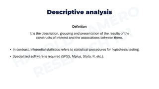
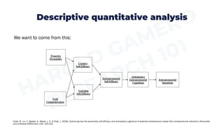
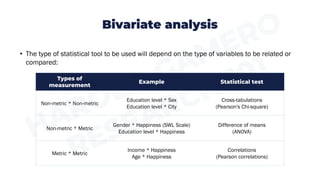
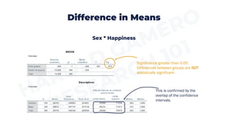
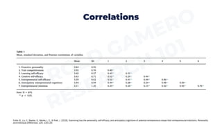
This document provides an overview of descriptive statistics and quantitative analysis. Descriptive statistics are used to describe and summarize data, and include frequency distributions, measures of central tendency (mean, median, mode), and measures of dispersion (range, standard deviation, variance). Univariate analysis examines one variable at a time using these descriptive statistics. Bivariate analysis examines the relationship between two variables using statistical tests like cross-tabulations, difference of means tests, and correlations depending on the type of variables. Specialized software is required to perform these analyses to gain insights from data in research studies.

1. Research 101: Quantitative Analysis -
Descriptive Statistics
Harold Gamero

2. Descriptive analysis
Definition
It is the description, grouping and presentation of the results of the
constructs of interest and the associations between them.
• In contrast, inferential statistics refers to statistical procedures for hypothesis testing.
• Specialized software is required (SPSS, Mplus, Stata, R, etc.).

3. Descriptive quantitative analysis
We want to come from this:
Fuller, B., Liu, Y., Bajaba, S., Marler, L. E., & Pratt, J. (2018). Examining how the personality, self-efficacy, and anticipatory cognitions of potential entrepreneurs shape their entrepreneurial intentions. Personality
and Individual Differences, 125, 120-125.

4. Descriptive quantitative analysis
To this:
Fuller, B., Liu, Y., Bajaba, S., Marler, L. E., & Pratt, J. (2018). Examining how the personality, self-efficacy, and anticipatory cognitions of potential entrepreneurs shape their
entrepreneurial intentions. Personality and Individual Differences, 125, 120-125.

5. Descriptive quantitative analysis
Through this:

6. Descriptive quantitative analysis
Using this (or similar programs):

7. Univariate Analysis
• The most basic statistical calculation.
• It helps to know the general configuration of our data.
• It includes 3 types of analysis:
a) Frequency distribution
b) Central tendency
c) Dispersion

8. Frequency Distribution
• Count of individual values per variable or response category and their respective
percentages.
• These values can be presented in tables and graphs (histograms).
• In large, random samples, histograms should follow the shape of a normal distribution
curve.
• Recommended for categorical variables (nominal or ordinal).
• It should not be used to analyse individual items of a composite measurement scale.

9. Frequency Distribution

10. Central Tendency
• They estimate the central values of a variable in our data.
• These measures are: Mean, mode, median.
• Means can be:
➢ Arithmetic: Sum of values / Number of values.
➢ Geometric: n-th root of the product of n values.
➢ Harmonic: Inverse of the arithmetic mean of the inverses of these values.
• In the social sciences, the arithmetic mean is mainly used.

11. Dispersion
• They indicate the variability of the sample data around the central tendency.
• Three common measures of dispersion are: range, standard deviation & variance.
• The range is especially sensitive to outliers.
• The standard deviation corrects for this effect by weighting the distances between the
values and the mean. It is also presented in the same units as the data (interpretable).
• The variance is the standard deviation squared. It is useful for mathematical procedures.

12. Bivariate analysis
• The type of statistical tool to be used will depend on the type of variables to be related or
compared:
Types of
measurement
Example Statistical test
Non-metric * Non-metric
Education level * Sex
Education level * City
Cross-tabulations
(Pearson's Chi-square)
Non-metric * Metric
Gender * Happiness (SWL Scale)
Education level * Happiness
Difference of means
(ANOVA)
Metric * Metric
Income * Happiness
Age * Happiness
Correlations
(Pearson correlations)

13. Cross Tables
Significance greater than 0.05
=
The differences between categories are
NOT statistically significant.
Education Level * Sex

14. Difference in Means
Sex * Happiness
Significance greater than 0.05
Differences between groups are NOT
statistically significant.
This is confirmed by the
overlap of the confidence
intervals.

15. Difference in Means
Age Bracket * Happiness
Significance less than 0.05
The differences between groups ARE
statistically significant.
People under 30 have
lower levels of happiness
than those aged 50 and
over.

16. Correlations
The data are reflected in
the table as in a
transverse mirror.
The asterisks represent the level of
statistical significance.

17. Correlations
These two data are
identical because they
are the same
correlation.
These correlations will
always be 1 since it is the
correlation of a variable
with itself.

18. Correlations
Usually the table is presented:
1. Showing only the lower half
2. Eliminating other values from the table such as N and sig.
3. Eliminating correlations between the same variables
4. Replacing variable names with numbers in the headers.

19. Correlations
Fuller, B., Liu, Y., Bajaba, S., Marler, L. E., & Pratt, J. (2018). Examining how the personality, self-efficacy, and anticipatory cognitions of potential entrepreneurs shape their entrepreneurial intentions. Personality
and Individual Differences, 125, 120-125.

20. Thank you.
Harold Gamero