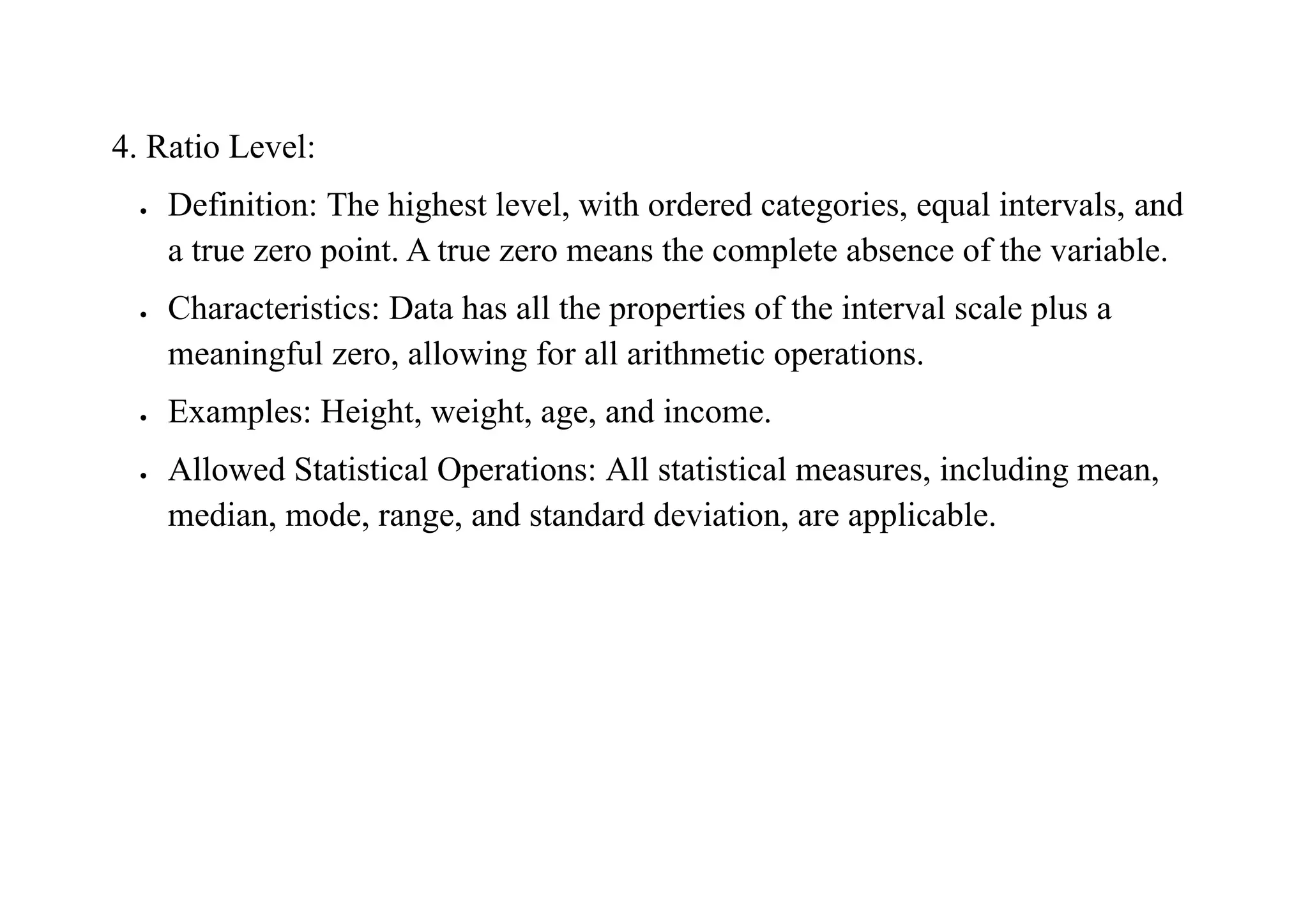
Basic Statistics in Social
Science Research
Your one-shot notes for better statistical understanding || For UGC NET/JRF
Contents
• Level Of Measurements
• Descriptive Statistics
• Inferential Statistics
• Key Statistical Tests in Social Science Research
o z- test; t-test; chi square test; ANOVA; Regression Analysis; Correlation Sampling, types, usage
• What is Skewed Data?
• Basic Sampling Terms
• Data Visualization Tools
Level Of Measurements
1. Nominal Level:
• Definition: This is the simplest level, used for categorizing data into
distinct groups without inherent order or ranking. Data can only be
labeled.
• Characteristics: Categories are mutually exclusive and represent
qualitative data with no inherent order or numerical value.
• Examples: Gender, religion, eye color, and marital status.
• Allowed Statistical Operations: Measures of frequency and the mode are
appropriate.
2. Ordinal Level:
• Definition: This level categorizes data into ranked or ordered categories,
but the differences between them are not necessarily equal or measurable.
• Characteristics: Data is ordered according to a criterion, but the intervals
between ranks are not uniform.
• Examples: Educational level, satisfaction levels, and military ranks.
• Allowed Statistical Operations: Frequency distributions, median, and
mode can be used, as well as measures of dispersion like percentiles.
3. Interval Level:
• Definition: This scale has ordered categories with equal intervals, but
it lacks a true zero point.
• Characteristics: Data can be categorized and ranked with consistent
intervals, but zero doesn't mean the absence of the attribute.
• Examples: Temperature in Celsius or Fahrenheit and IQ scores.
• Allowed Statistical Operations: Mode, median, and mean can be used,
along with measures of dispersion like standard deviation.
4. Ratio Level:
• Definition: The highest level, with ordered categories, equal intervals, and
a true zero point. A true zero means the complete absence of the variable.
• Characteristics: Data has all the properties of the interval scale plus a
meaningful zero, allowing for all arithmetic operations.
• Examples: Height, weight, age, and income.
• Allowed Statistical Operations: All statistical measures, including mean,
median, mode, range, and standard deviation, are applicable.
Descriptive Statistics
Used to summarize and describe data.
a. Measures of Central Tendency
• Mean: Arithmetic average.
• Median: Middle value in ordered data.
• Mode: Most frequent value.
Mean (Average)
Mean is what we usually call average.
How to find it:
• Add all the numbers together.
• Divide the total by how many numbers there are.
Example:
Let’s say your scores in 5 tests are:
80, 90, 70, 60, 100
Add them up:
80 + 90 + 70 + 60 + 100 = 400
Now divide by 5:
400 ÷ 5 = 80
Mean = 80
2. Median (Middle Number)
Median is the middle number when the numbers are in order.
How to find it:
• Arrange the numbers from small to big.
• Find the number in the middle.
Example:
Numbers: 90, 60, 100, 70, 80
Step 1: Put them in order:
60, 70, 80, 90, 100
Step 2: Find the middle one:
Median = 80
If there are two numbers in the middle, take their average!
Mode (Most Often)
Mode is the number that appears the most.
Example:
If your scores are:
70, 80, 80, 90, 100
80 appears twice, more than any other number.
Mode = 80
If no number repeats, then there is no mode.
Summary Table
Term What it Means How to Find It
Mean Average Add all and divide by how many numbers
MedianMiddle number Order numbers, pick the center one
Mode Most frequent numberFind the number that shows up the most
b. Measures of Dispersion
• Range: Max - Min.
• Variance: Average of squared deviations from the mean.
• Standard Deviation (SD): Square root of variance.
• Coefficient of Variation (CV): CV = (σ / μ) × 100
𝐶𝑜𝑒𝑓𝑓𝑖𝑐𝑖𝑒𝑛𝑡 𝑜𝑓 𝑉𝑎𝑟𝑖𝑎𝑡𝑖𝑜𝑛 (𝐶𝑉)
= (𝑆𝑡𝑎𝑛𝑑𝑎𝑟𝑑 𝐷𝑒𝑣𝑖𝑎𝑡𝑖𝑜𝑛 ÷ 𝑀𝑒𝑎𝑛) × 100
Inferential Statistics
Used to make predictions or test hypotheses based on sample data.
a. Hypothesis Testing
• Null Hypothesis (H₀): No effect or difference.
• Alternative Hypothesis (H₁): There is an effect or difference.
b. Significance Level (α)
• Common levels: 0.05, 0.01
• If p-value < α → reject H₀
Key Statistical Tests in Social Science Research
Statistical tests help researchers analyze data and draw conclusions about
populations. Below is an overview of the most commonly used statistical tests
in social science, along with illustrative examples.
t-test
Purpose: To determine whether the means of two groups are significantly
different.
Types:
• Independent t-test: Compares two different groups.
• Paired t-test: Compares the same group at two time points.
Example 1 – Independent t-test: A researcher wants to evaluate whether male
and female students differ in their levels of academic stress. A sample of 30
males and 30 females is taken, and their stress scores are measured using a
standardized scale. The t-test is used to compare the average scores between
the two groups.
Example 2 – Paired t-test: A psychologist implements a mindfulness training
program for students with exam anxiety. The anxiety levels of students are
measured before and after the program. A paired t-test determines whether the
change is statistically significant.
ANOVA (Analysis of Variance)
Purpose: To compare the means of three or more groups to determine if at least
one differs significantly.
Types:
• One-way ANOVA: One independent variable with multiple groups.
• Two-way ANOVA: Two independent variables studied simultaneously.
Example 1 – One-way ANOVA: A sociologist studies the effect of
socioeconomic background (low, middle, high income) on attitudes toward
political participation. ANOVA helps determine if there are significant
differences in attitudes among the three groups.
Example 2 – Two-way ANOVA: An education researcher wants to know if
both gender (male/female) and teaching style (traditional/interactive)
influence students’academic performance. A two-way ANOVA is applied to
assess the individual and combined effects of both variables.
Chi-square Test (χ²)
Purpose: To examine the relationship between two categorical variables.
Types:
• Test of independence: Checks if two variables are related.
• Goodness-of-fit test: Checks if data fits expected distribution.
Example 1 – Test of Independence: A political analyst wants to know whether
voting preference (Party A, B, or C) is associated with gender (male/female). A
chi-square test of independence is used to determine if the association is
statistically significant.
Example 2 – Goodness-of-Fit: A researcher surveys whether people prefer four
types of news media (TV, radio, newspapers, online). If the researcher assumes
equal preference for each but finds that online media dominates, a chi-square
goodness-of-fit test checks if the observed preferences deviate significantly
from expectations.
Z-test
Purpose: To test whether a sample mean significantly differs from a known
population mean. It is typically used when the sample size is large (n > 30) and
the population variance is known.
Example: A government economist wants to check if the average monthly
household income in a specific town (₹28,000) is significantly different from
the national average (₹25,000). Since the population standard deviation is
known and the sample size is 100, a z-test is applied.
Correlation (r)
Purpose: To assess the degree and direction of association between two
continuous variables.
Interpretation:
• r = +1: Perfect positive correlation
• r = 0: No correlation
• r = -1: Perfect negative correlation
Example 1: A researcher studies the relationship between the number of hours
students spend on social media per day and their academic grades. A negative
correlation would suggest that more screen time is associated with lower
grades.
Example 2: A public health researcher examines the relationship between daily
physical activity (minutes) and mental well-being scores among working
adults. A positive correlation would support the idea that more exercise is
associated with better mental health.
Regression Analysis
Purpose: To predict the value of one variable (dependent variable) based on
one or more other variables (independent variables). It also helps in
understanding the strength and nature of influence.
Types:
• Simple linear regression: One predictor variable
• Multiple regression: Two or more predictor variables
Example 1 – Simple Regression: A sociologist wants to predict an individual's
life satisfaction score based on their income level. Simple linear regression is
used to assess how income influences satisfaction.
Example 2 – Multiple Regression: A researcher explores the factors that
predict college dropout rates. Independent variables include parental
education, financial support, high school grades, and stress levels. Multiple
regression analysis reveals which factors have the strongest influence.
Summary Table
Test Use Case Data Type
Common Application in
Social Science
t-test
Compare means of 2
groups
Continuous
Gender difference in
exam performance
ANOVA
Compare means of 3+
groups
Continuous
Comparing political
attitudes by education
level
Test Use Case Data Type
Common Application in
Social Science
Chi-square
Test relationship
between categories
Categorical
Association between
gender and voting
preference
Z-test
Compare sample mean
with population mean
Continuous
(large sample)
Checking if local income
differs from national
mean
Correlation
(r)
Measure relationship
strength
Continuous
Social media time vs
academic score
Regression
Predict dependent
variable
Continuous
Predicting dropout based
on stress, finances, etc.
Correlation vs. Causation
• Correlation: A mutual relationship (e.g., income and education).
• Causation: One variable directly affects another (e.g., smoking causes
cancer).
Sampling
Sampling is the process of selecting a small group (sample) from a larger
group (population) to study. Instead of collecting data from every single person
in a population (which is time-consuming and expensive), researchers collect
data from a representative few, and then make inferences about the whole.
Why Use Sampling?
• Saves time and money
• Easier to manage and study
• Can still give accurate results if done properly
Basic Sampling Terms You Must Know
Term
• Population
• Sample
• Sampling
Frame
• Unit
Meaning
• The whole group you're studying (e.g., all college
students in India)
• A part of the population chosen for the actual study
• The list from which the sample is drawn (e.g., a list of
all students)
• A single member of the population (e.g., one student)
Types of Sampling
A. Probability Sampling
Mehtod Description When to Use
1. Simple
Random
Sampling
Randomly pick units (like a
lottery draw)
When population is small and
well-defined
2. Systematic
Sampling
Pick every nth person from a
list (e.g., every 10th name)
When a list is available and well
ordered
3. Stratified
Sampling
Divide population into groups
(strata) and sample from each
When you want all subgroups
(e.g., male/female) represented
4. Cluster
Sampling
Divide into clusters, then
randomly pick whole clusters
Useful for large and
geographically spread-out
populations
B. Non-Probability Sampling
Method Description Example Use Case
1. Convenience
Sampling
Pick whoever is easiest to reach
Online surveys, student
research
2. Purposive
Sampling
Choose people based on a
specific purpose/criteria
Interviewing teachers
about education
3. Snowball
Sampling
Existing participants refer new
participants
Hard-to-reach groups
(e.g., drug users)
4. Quota
Sampling
Choose a set number of
participants from each category
Ensuring equal males and
females in sample
Characteristics Of Good Sampling And Bad Sampling
Good Sample Bad Sample
Representative of the population Biased or too narrow
Randomly chosen (in probability sampling) Based only on convenience
Diverse and inclusive Missing important sub-groups
Data Visualization Tools
• Bar Chart: Compares categorical data using bars. (e.g., sales across
regions)
• Histogram: Visualizes frequency distribution of continuous numerical
data. (e.g., distribution of test scores)
• Pie Chart: Shows proportions of a whole using slices. (e.g., budget
allocation)
• Scatter Plot: Shows the relationship between two numerical variables.
(e.g., height vs. weight)
What is Skewed Data?
Skewed data means the data is not evenly distributed — it's lopsided or
stretched more on one side than the other.
In other words, most of the values are bunched up on one side, and there’s a
long tail on the other.
Types of Skewed Data
1. Right Skewed (Positively Skewed)
• The tail is on the right (towards larger values).
• A few big numbers pull the mean up.
Example: Incomes in a city — most people earn ₹20,000–₹30,000, but a few
earn ₹1 crore.
2. Left Skewed (Negatively Skewed)
• The tail is on the left (towards smaller values).
• A few small numbers pull the mean down.
Example: Age at retirement — most people retire around 60–65, but a few
retire early at 40.
Why Skewness Matters
• It tells us if mean is a good measure or not.
• In skewed data, the median is often a better measure of central tendency
than the mean.
• Helps in choosing the right statistical tests and interpretation.
Skew Type
Tail
Direction
Best
Measure
Real-Life Example
Right Skew
(Positive)
Right Median Income, property prices
Left Skew
(Negative)
Left Median
Exam scores (if most do
well)

Basic Statistics in Social Science Research.pdf

  • 1.
    Basic Statistics inSocial Science Research Your one-shot notes for better statistical understanding || For UGC NET/JRF Contents • Level Of Measurements • Descriptive Statistics • Inferential Statistics • Key Statistical Tests in Social Science Research o z- test; t-test; chi square test; ANOVA; Regression Analysis; Correlation Sampling, types, usage • What is Skewed Data? • Basic Sampling Terms • Data Visualization Tools
  • 2.
    Level Of Measurements 1.Nominal Level: • Definition: This is the simplest level, used for categorizing data into distinct groups without inherent order or ranking. Data can only be labeled. • Characteristics: Categories are mutually exclusive and represent qualitative data with no inherent order or numerical value. • Examples: Gender, religion, eye color, and marital status. • Allowed Statistical Operations: Measures of frequency and the mode are appropriate. 2. Ordinal Level: • Definition: This level categorizes data into ranked or ordered categories, but the differences between them are not necessarily equal or measurable.
  • 3.
    • Characteristics: Datais ordered according to a criterion, but the intervals between ranks are not uniform. • Examples: Educational level, satisfaction levels, and military ranks. • Allowed Statistical Operations: Frequency distributions, median, and mode can be used, as well as measures of dispersion like percentiles. 3. Interval Level: • Definition: This scale has ordered categories with equal intervals, but it lacks a true zero point. • Characteristics: Data can be categorized and ranked with consistent intervals, but zero doesn't mean the absence of the attribute. • Examples: Temperature in Celsius or Fahrenheit and IQ scores. • Allowed Statistical Operations: Mode, median, and mean can be used, along with measures of dispersion like standard deviation.
  • 4.
    4. Ratio Level: •Definition: The highest level, with ordered categories, equal intervals, and a true zero point. A true zero means the complete absence of the variable. • Characteristics: Data has all the properties of the interval scale plus a meaningful zero, allowing for all arithmetic operations. • Examples: Height, weight, age, and income. • Allowed Statistical Operations: All statistical measures, including mean, median, mode, range, and standard deviation, are applicable.
  • 5.
    Descriptive Statistics Used tosummarize and describe data. a. Measures of Central Tendency • Mean: Arithmetic average. • Median: Middle value in ordered data. • Mode: Most frequent value. Mean (Average) Mean is what we usually call average. How to find it: • Add all the numbers together. • Divide the total by how many numbers there are.
  • 6.
    Example: Let’s say yourscores in 5 tests are: 80, 90, 70, 60, 100 Add them up: 80 + 90 + 70 + 60 + 100 = 400 Now divide by 5: 400 ÷ 5 = 80 Mean = 80 2. Median (Middle Number) Median is the middle number when the numbers are in order. How to find it: • Arrange the numbers from small to big.
  • 7.
    • Find thenumber in the middle. Example: Numbers: 90, 60, 100, 70, 80 Step 1: Put them in order: 60, 70, 80, 90, 100 Step 2: Find the middle one: Median = 80 If there are two numbers in the middle, take their average! Mode (Most Often) Mode is the number that appears the most. Example: If your scores are: 70, 80, 80, 90, 100
  • 8.
    80 appears twice,more than any other number. Mode = 80 If no number repeats, then there is no mode. Summary Table Term What it Means How to Find It Mean Average Add all and divide by how many numbers MedianMiddle number Order numbers, pick the center one Mode Most frequent numberFind the number that shows up the most
  • 9.
    b. Measures ofDispersion • Range: Max - Min. • Variance: Average of squared deviations from the mean. • Standard Deviation (SD): Square root of variance. • Coefficient of Variation (CV): CV = (σ / μ) × 100 𝐶𝑜𝑒𝑓𝑓𝑖𝑐𝑖𝑒𝑛𝑡 𝑜𝑓 𝑉𝑎𝑟𝑖𝑎𝑡𝑖𝑜𝑛 (𝐶𝑉) = (𝑆𝑡𝑎𝑛𝑑𝑎𝑟𝑑 𝐷𝑒𝑣𝑖𝑎𝑡𝑖𝑜𝑛 ÷ 𝑀𝑒𝑎𝑛) × 100
  • 10.
    Inferential Statistics Used tomake predictions or test hypotheses based on sample data. a. Hypothesis Testing • Null Hypothesis (H₀): No effect or difference. • Alternative Hypothesis (H₁): There is an effect or difference. b. Significance Level (α) • Common levels: 0.05, 0.01 • If p-value < α → reject H₀ Key Statistical Tests in Social Science Research Statistical tests help researchers analyze data and draw conclusions about populations. Below is an overview of the most commonly used statistical tests in social science, along with illustrative examples.
  • 11.
    t-test Purpose: To determinewhether the means of two groups are significantly different. Types: • Independent t-test: Compares two different groups. • Paired t-test: Compares the same group at two time points. Example 1 – Independent t-test: A researcher wants to evaluate whether male and female students differ in their levels of academic stress. A sample of 30 males and 30 females is taken, and their stress scores are measured using a standardized scale. The t-test is used to compare the average scores between the two groups. Example 2 – Paired t-test: A psychologist implements a mindfulness training program for students with exam anxiety. The anxiety levels of students are
  • 12.
    measured before andafter the program. A paired t-test determines whether the change is statistically significant. ANOVA (Analysis of Variance) Purpose: To compare the means of three or more groups to determine if at least one differs significantly. Types: • One-way ANOVA: One independent variable with multiple groups. • Two-way ANOVA: Two independent variables studied simultaneously. Example 1 – One-way ANOVA: A sociologist studies the effect of socioeconomic background (low, middle, high income) on attitudes toward political participation. ANOVA helps determine if there are significant differences in attitudes among the three groups.
  • 13.
    Example 2 –Two-way ANOVA: An education researcher wants to know if both gender (male/female) and teaching style (traditional/interactive) influence students’academic performance. A two-way ANOVA is applied to assess the individual and combined effects of both variables. Chi-square Test (χ²) Purpose: To examine the relationship between two categorical variables. Types: • Test of independence: Checks if two variables are related. • Goodness-of-fit test: Checks if data fits expected distribution. Example 1 – Test of Independence: A political analyst wants to know whether voting preference (Party A, B, or C) is associated with gender (male/female). A chi-square test of independence is used to determine if the association is statistically significant.
  • 14.
    Example 2 –Goodness-of-Fit: A researcher surveys whether people prefer four types of news media (TV, radio, newspapers, online). If the researcher assumes equal preference for each but finds that online media dominates, a chi-square goodness-of-fit test checks if the observed preferences deviate significantly from expectations. Z-test Purpose: To test whether a sample mean significantly differs from a known population mean. It is typically used when the sample size is large (n > 30) and the population variance is known. Example: A government economist wants to check if the average monthly household income in a specific town (₹28,000) is significantly different from the national average (₹25,000). Since the population standard deviation is known and the sample size is 100, a z-test is applied.
  • 15.
    Correlation (r) Purpose: Toassess the degree and direction of association between two continuous variables. Interpretation: • r = +1: Perfect positive correlation • r = 0: No correlation • r = -1: Perfect negative correlation Example 1: A researcher studies the relationship between the number of hours students spend on social media per day and their academic grades. A negative correlation would suggest that more screen time is associated with lower grades. Example 2: A public health researcher examines the relationship between daily physical activity (minutes) and mental well-being scores among working
  • 16.
    adults. A positivecorrelation would support the idea that more exercise is associated with better mental health. Regression Analysis Purpose: To predict the value of one variable (dependent variable) based on one or more other variables (independent variables). It also helps in understanding the strength and nature of influence. Types: • Simple linear regression: One predictor variable • Multiple regression: Two or more predictor variables Example 1 – Simple Regression: A sociologist wants to predict an individual's life satisfaction score based on their income level. Simple linear regression is used to assess how income influences satisfaction.
  • 17.
    Example 2 –Multiple Regression: A researcher explores the factors that predict college dropout rates. Independent variables include parental education, financial support, high school grades, and stress levels. Multiple regression analysis reveals which factors have the strongest influence. Summary Table Test Use Case Data Type Common Application in Social Science t-test Compare means of 2 groups Continuous Gender difference in exam performance ANOVA Compare means of 3+ groups Continuous Comparing political attitudes by education level
  • 18.
    Test Use CaseData Type Common Application in Social Science Chi-square Test relationship between categories Categorical Association between gender and voting preference Z-test Compare sample mean with population mean Continuous (large sample) Checking if local income differs from national mean Correlation (r) Measure relationship strength Continuous Social media time vs academic score Regression Predict dependent variable Continuous Predicting dropout based on stress, finances, etc.
  • 19.
    Correlation vs. Causation •Correlation: A mutual relationship (e.g., income and education). • Causation: One variable directly affects another (e.g., smoking causes cancer). Sampling Sampling is the process of selecting a small group (sample) from a larger group (population) to study. Instead of collecting data from every single person in a population (which is time-consuming and expensive), researchers collect data from a representative few, and then make inferences about the whole. Why Use Sampling? • Saves time and money • Easier to manage and study • Can still give accurate results if done properly
  • 20.
    Basic Sampling TermsYou Must Know Term • Population • Sample • Sampling Frame • Unit Meaning • The whole group you're studying (e.g., all college students in India) • A part of the population chosen for the actual study • The list from which the sample is drawn (e.g., a list of all students) • A single member of the population (e.g., one student)
  • 21.
    Types of Sampling A.Probability Sampling Mehtod Description When to Use 1. Simple Random Sampling Randomly pick units (like a lottery draw) When population is small and well-defined 2. Systematic Sampling Pick every nth person from a list (e.g., every 10th name) When a list is available and well ordered 3. Stratified Sampling Divide population into groups (strata) and sample from each When you want all subgroups (e.g., male/female) represented 4. Cluster Sampling Divide into clusters, then randomly pick whole clusters Useful for large and geographically spread-out populations
  • 22.
    B. Non-Probability Sampling MethodDescription Example Use Case 1. Convenience Sampling Pick whoever is easiest to reach Online surveys, student research 2. Purposive Sampling Choose people based on a specific purpose/criteria Interviewing teachers about education 3. Snowball Sampling Existing participants refer new participants Hard-to-reach groups (e.g., drug users) 4. Quota Sampling Choose a set number of participants from each category Ensuring equal males and females in sample
  • 23.
    Characteristics Of GoodSampling And Bad Sampling Good Sample Bad Sample Representative of the population Biased or too narrow Randomly chosen (in probability sampling) Based only on convenience Diverse and inclusive Missing important sub-groups
  • 24.
    Data Visualization Tools •Bar Chart: Compares categorical data using bars. (e.g., sales across regions) • Histogram: Visualizes frequency distribution of continuous numerical data. (e.g., distribution of test scores) • Pie Chart: Shows proportions of a whole using slices. (e.g., budget allocation) • Scatter Plot: Shows the relationship between two numerical variables. (e.g., height vs. weight)
  • 25.
    What is SkewedData? Skewed data means the data is not evenly distributed — it's lopsided or stretched more on one side than the other. In other words, most of the values are bunched up on one side, and there’s a long tail on the other. Types of Skewed Data 1. Right Skewed (Positively Skewed) • The tail is on the right (towards larger values). • A few big numbers pull the mean up. Example: Incomes in a city — most people earn ₹20,000–₹30,000, but a few earn ₹1 crore. 2. Left Skewed (Negatively Skewed)
  • 26.
    • The tailis on the left (towards smaller values). • A few small numbers pull the mean down. Example: Age at retirement — most people retire around 60–65, but a few retire early at 40. Why Skewness Matters • It tells us if mean is a good measure or not. • In skewed data, the median is often a better measure of central tendency than the mean. • Helps in choosing the right statistical tests and interpretation.
  • 27.
    Skew Type Tail Direction Best Measure Real-Life Example RightSkew (Positive) Right Median Income, property prices Left Skew (Negative) Left Median Exam scores (if most do well)