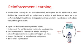
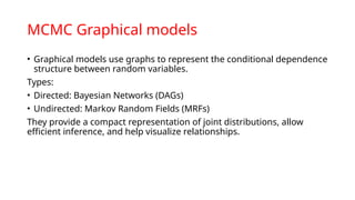
Reinforcement Learning–(Q-Learning, Deep Q-Networks) – Transfer Learning and Pretrained Models – Markov Chain Monte Carlo Methods – Sampling – Proposal Distribution – Markov Chain Monte Carlo – Graphical Models – Bayesian Networks – Markov Random Fields – Case Studies: Real-World Machine Learning Applications – Future Trends in Machine Learning

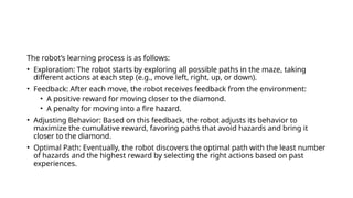
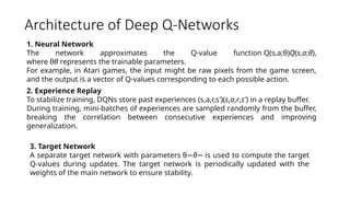
![Loss Function
•The loss function measures the difference between the
predicted Q-values and the target Q-values:
L(θ)=E[(r+γmaxa’
Q(s’,a’;θ )–
− Q(s,a;θ))2]](https://image.slidesharecdn.com/unit-5-250614155909-fe4034be/85/R22-Machine-learning-jntuh-UNIT-5-pptx-16-320.jpg)


![house price prediction w2_batc_4[1].pptx](https://cdn.slidesharecdn.com/ss_thumbnails/w2batc41-250509135959-1eb87be6-thumbnail.jpg?width=640&height=640&fit=bounds)


