Download as PDF, PPTX

![18/59
Reward
I The reward Rt ∈ R at time t is a numerical (scalar) feedback signal the environment
emits based on the agent’s action and the state it was in and moved to.
I Rt = R(St, At, St+1), R : S × A × S → R
I The reward can be received instantaneously or is delayed.
I A key hypothesis in reinforcement learning is the Reward Hypothesis which states that
all goals can be described by the maximisation of expected cumulative reward.
I The return Gt is the total discounted (or undiscounted) reward starting from time step t
Gt = Rt+1 + γRt+2 + γ2
Rt+3 + . . . =
∞
X
k=0
γk
Rt+k+1 (3)
I γ ∈ [0, 1] is the discount factor representing the assigned present value of future rewards.
I Examples:
I PnL (profit and loss)
I Sharpe ratio](https://image.slidesharecdn.com/rlinfinancelecture2021-210310205230/75/Reinforcement-Learning-for-Financial-Markets-18-2048.jpg)
![19/59
Markov Decision Process (1/3)
I Markov decision processes (MDP) describes a fully observable environment for the
reinforcement learning paradigm.
I Reinforcement Learning problems are typically formalised as an MDP.
I A key property is the Markov property:
P [St+1 | S1, . . . , St] = P [St+1 | St] (4)
I The state transition probability for a Markov state s and a successor state s0
is defined
by:
Pss0 = P [St+1 = s0
| St = s] (5)
I This can be defined in a matrix form with the state transition probability matrix P
describing the transition probabilities from all states s to all successor states s0
P =
P11 . . . P1n
.
.
.
Pn1 . . . Pnn
(6)](https://image.slidesharecdn.com/rlinfinancelecture2021-210310205230/75/Reinforcement-Learning-for-Financial-Markets-19-2048.jpg)
![20/59
Markov Decision Process (2/3)
I A Markov Process (Markov Chain) is a tuple hS, Pi of random states S1, S2, . . . with
the Markov property.
I A Markov Reward Process is a tuple hS, P, R, γi
I A Markov Decision Process is an extension of the Markov reward process with decisions
in which all the states are Markov. It is a tuple hS, A, P, R, γi where,
I S is a finite set of states
I A is a finite set of actions
I P is a state transition probability matrix, Pa
ss0 = P [St+1 = s0
| St = s, At = a]
I R is a reward function, Ra
s = E [Rt+1 | St = s, At = a]
I γ is a discount factor, γ ∈ [0, 1]](https://image.slidesharecdn.com/rlinfinancelecture2021-210310205230/75/Reinforcement-Learning-for-Financial-Markets-20-2048.jpg)
![21/59
Markov Decision Process (3/3)
I Many extensions to MDP exist. These include, for example, Partially observable MDPs
I A Partially Observable Markov Decision Process is an extension of the Markov
decision process with hidden states. It is a tuple hS, A, O, P, R, Z, γi where,
I S is a finite set of states
I A is a finite set of actions
I O is a finite set of observations
I P is a state transition probability matrix, Pa
ss0 = P [St+1 = s0
| St = s, At = a]
I R is a reward function, Ra
s = E [Rt+1 | St = s, At = a]
I Z is an observation function, Za
s0o = P [Ot+1 = o | St+1 = s0
, At = a]
I γ is a discount factor, γ ∈ [0, 1]](https://image.slidesharecdn.com/rlinfinancelecture2021-210310205230/75/Reinforcement-Learning-for-Financial-Markets-21-2048.jpg)
![22/59
Policy
I The policy π is the function that fully defines the agent’s behaviour. The policy is
essentially what we’re trying to learn in reinforcement learning.
I A policy can be described as a mapping from state to actions π : S → A. More formally,
the policy π is a distribution over actions given states.
I It can be deterministic At+1 = π (St) or stochastic π(a | s) = P [At = a | St = s]
I Policies are stationary (time-independent), At+1 ∼ π (· | St) , ∀t > 0](https://image.slidesharecdn.com/rlinfinancelecture2021-210310205230/75/Reinforcement-Learning-for-Financial-Markets-22-2048.jpg)
![23/59
Value Function
I The value function is another important function that describes how good/bad it is to
be in a current state and/or taking a particular action. More formally, it is a prediction of
future rewards and gives the long-term value of the state s and action a.
I Remember, the return Gt is the total discounted reward starting from time step t
Gt = Rt+1 + γRt+2 + γ2
Rt+3 + . . . =
∞
X
k=0
γk
Rt+k+1 (7)
I The state-value function vπ(s) of an MDP is the expected return starting from state s,
and then following policy π
vπ(s) = Eπ [Gt | St = s] = Eπ
Rt+1 + γRt+2 + γ2
Rt+3 + . . . | St = s
(8)
I The action-value function qπ(s, a) of an MDP is the expected return starting from state
s, taking action a, and then following policy π
qπ(s, a) = Eπ [Gt | St = s, At = a] = Eπ
Rt+1 + γRt+2 + γ2
Rt+3 + . . . | St = s, At = a
(9)](https://image.slidesharecdn.com/rlinfinancelecture2021-210310205230/75/Reinforcement-Learning-for-Financial-Markets-23-2048.jpg)
![24/59
Bellman Expectation Equation
I The state-value function can be decomposed into two components: (1) the immediate
reward Rt+1 and (2) the discounted value of the successor state γvπ(St+1)
vπ(s) = Eπ [Gt | St = s]
= Eπ
Rt+1 + γRt+2 + γ2
Rt+3 + . . . | St = s
= Eπ [Rt+1 + γ (Rt+2 + γRt+3 + . . .) | St = s]
= Eπ [Rt+1 + γGt+1 | St = s]
= Eπ [Rt+1 + γvπ (St+1) | St = s]
(10)
I Similarly, the action-value function can be decomposed to:
qπ(s, a) = Eπ [Rt+1 + γqπ (St+1, At+1) | St = s, At = a] (11)](https://image.slidesharecdn.com/rlinfinancelecture2021-210310205230/75/Reinforcement-Learning-for-Financial-Markets-24-2048.jpg)
![36/59
Policy Gradient
I Policy gradient methods attempt to learn
a parameterised policy directly instead of
generating the policy from the value
function (e.g. using -greedy)
πθ(s, a) = P[a | s, θ] (23)
I The goal is to find the best parameters θ
that maximizes J(θ)
I Policy gradient methods search for a local
maximum in J(θ) by ascending the
gradient of the policy w.r.t to θ
∆θ = α∇θJ(θ) (24)
I Policy Gradient Theorem:
∇θJ(θ) = Eπθ
[∇θ log πθ(s, a)Qπθ
(s, a)]
(25)](https://image.slidesharecdn.com/rlinfinancelecture2021-210310205230/75/Reinforcement-Learning-for-Financial-Markets-36-2048.jpg)

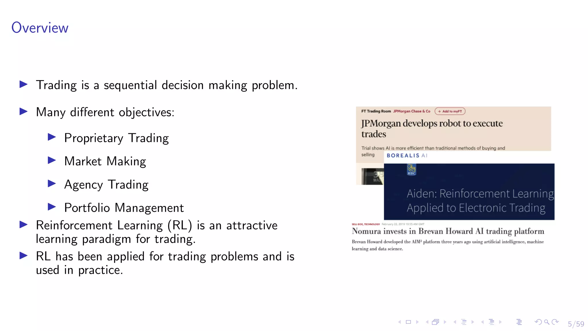
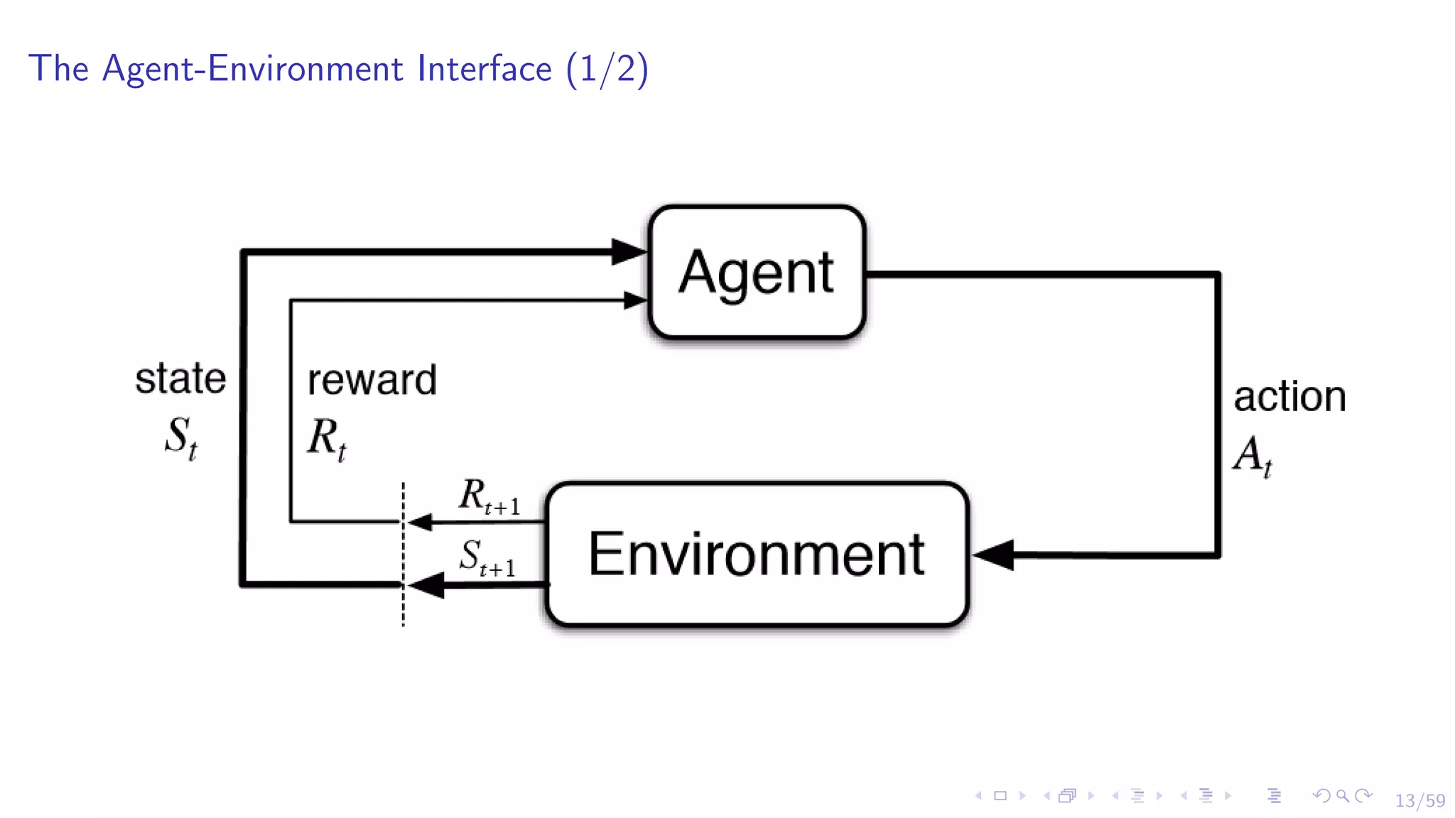
The document discusses the application of reinforcement learning (RL) in financial markets, detailing its advantages, key algorithms, and challenges. It describes RL as a sequential decision-making approach suitable for various trading objectives, such as proprietary trading and portfolio management. The authors emphasize the importance of understanding the algorithms and methodologies behind RL while also acknowledging that the document is for informational purposes and not investment advice.


![[역기획]승리의 여신 니케_전투 시스템](https://cdn.slidesharecdn.com/ss_thumbnails/random-240612074027-b21b1225-thumbnail.jpg?width=640&height=640&fit=bounds)