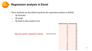
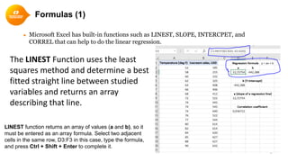
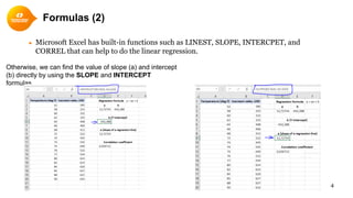
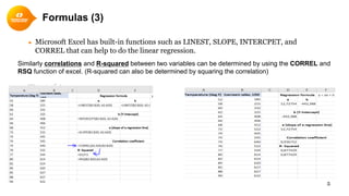
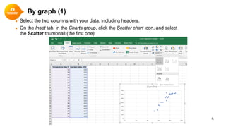
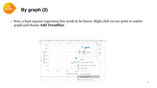
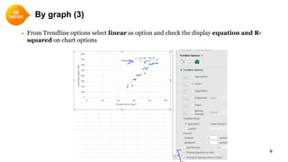
This document describes how to perform simple linear regression analysis in Microsoft Excel using three methods: formulas, graphs, and the built-in data analysis tool. It provides examples of how to use functions like LINEST, SLOPE, INTERCEPT, and CORREL to calculate the regression line and coefficients. It also demonstrates how to add a trendline to a scatter plot graph and use the data analysis tool to output regression statistics and residuals.
Introduces and explains the use of multiple linear regression, a multivariate correlational statistical technique. For more info, see the lecture page at http://goo.gl/CeBsv. See also the slides for the MLR II lecture http://www.slideshare.net/jtneill/multiple-linear-regression-ii
Regression Analysis is simplified in this presentation. Starting with simple linear to multiple regression analysis, it covers all the statistics and interpretation of various diagnostic plots. Besides, how to verify regression assumptions and some advance concepts of choosing best models makes the slides more useful SAS program codes of two examples are also included.
Simple Linear Regression: Step-By-StepDan Wellisch
This presentation was made to our meetup group found here.: https://www.meetup.com/Chicago-Technology-For-Value-Based-Healthcare-Meetup/ on 9/26/2017. Our group is focused on technology applied to healthcare in order to create better healthcare.
In this tutorial, we discuss how to do a regression analysis in Excel. I will teach you how to activate the regression analysis feature, what are the functions and methods we can use to do a regression analysis in Excel and most importantly, how to interpret the regression analysis results. Source: https://tinytutes.com/tutorials/regression-analysis-in-excel/
Exploring Support Vector Regression - Signals and Systems ProjectSurya Chandra
Our team competed in a Kaggle competition to predict the bike share use as a part of their capital bike share program in Washington DC using a powerful function approximation technique called support vector regression.
How to combine interpolation and regression graphs in RDougLoqa
This is a general tutorial that shows you how to take Census data, aggregate columns/rows and use interpolation lines and regression curves in your graphs. You can graph individual rows/columns or aggregate rows/columns. There is an example of graphs created here: https://www.linkedin.com/pulse/comparison-annual-income-going-back-from-2017-doug-loqa-doug-loqa/
Elementary Data Analysis with MS Excel_Day-5Redwan Ferdous
This event took place on 16th September 2020. This was arranged by EMK Center (Makerlab). The title was 'Elementary Data Analysis with MS Excel', where very basic data analysis with MS excel was discussed.
In Day-5, Hypothesis, Statistics, Regression Analysis, T-Test, Z-test, P-Test, ANOVA, Goal Seek, Pivot Chart, Dashboard, Slicer, Solver, Data Analysis Toolpak, and peripheral items were discussed.
Isotonic Regression is a statistical technique of fitting a free-form line to a sequence of observations such that the fitted line is non-decreasing (or non-increasing) everywhere, and lies as close to the observations as possible. Isotonic Regression is limited to predicting numeric output so the dependent variable must be numeric in nature…
Dimensionality Reduction and feature extraction.pptxSivam Chinna
Dimensionality reduction, or dimension reduction, is the transformation of data from a high-dimensional space into a low-dimensional space so that the low-dimensional representation retains some meaningful properties of the original data, ideally close to its intrinsic dimension.
ENGR 102B Microsoft Excel Proficiency LevelsPlease have your in.docxYASHU40
ENGR 102B: Microsoft Excel Proficiency Levels
Please have your instructor or TA initial each level as you complete it. If you need additional help, ask the TAs or use the help guide within Excel.
Once you master Excel Levels I through IV, you can note Excel as a skill on your resume!
Please see D2L Content for this week for your Excel Homework assignment (individual), which is due via D2L Dropbox by the due date specified in the D2L News for your section.
If you use a Mac, please be sure to submit your homework in a format that the grader and instructor can open on a PC.
Level I: Basic Functions Initials _______
1. Calculating an Average: Calculate the arithmetic average of the 5 values listed below. Enter the values in cells A2 through A6. Place a descriptive label in cell A1.
3.6, 3.8, 3.5, 3.7, 3.6
First, calculate the average the long way, by summing the values and dividing by 5:
You will enter the following formula into a blank cell to accomplish this:
=(A2+A3+A4+A5+A6)/5
Second, calculate the average using Excel’s AVERAGE( ) function by entering the following formula in a cell:
=AVERAGE(cellrange)
Replace the “cellrange” with the actual addresses in your spreadsheet of the range of cells holding the five values (i.e., for this problem, the cell range is A2:A6).
2. Determining Velocities (in kph): Some friends at the University of Calgary are coming south for spring break. Help them avoid a speeding ticket by completing a velocity conversion worksheet that calculates the conversion from mph to kph in increments of 10 from 10 to 100. A conversion factor you will need is 0.62 miles/km; you will need this factor to convert from miles/hour to km/hour. Place the conversion factor in its own cell and then reference it in your conversion calculations using absolute cell referencing (e.g., $C$2). Refer to the CBT video on Absolute and Relative Cell Referencing from the “Preparation for the Excel Workshop” assignment if you don’t remember how to do this.
Level II: Advanced Functions Initials _______
1. Projectile Motion I: (See following page for Fig. 1 Excel chart) A projectile is launched at the angle 35o from the horizontal with a velocity equal to 30 m/s. Neglecting air resistance and assuming a horizontal surface, determine how far away from the launch site the projectile will land.
To answer this problem, you will need:
1. Excel’s trigonometry functions to handle the 35o angle, and
2. Equations relating distance to velocity and acceleration
When velocity is constant, as in the horizontal motion of our particle (since we’re neglecting air resistance), the distance traveled is simply the initial horizontal velocity times the time of flight:
(Equation 1)
What keeps the projectile from flying forever is gravity. Since the gravitational acceleration is constant, the vertical distance traveled becomes
(Equation 2)
Because the projectile ends up back on the ground, the final value of y is zero (a hor ...
X‾ -R Chart maximum utilization of information available from data & provide detailed information in process average & variation for control of individual dimensions.
MAT 240 Random Sampling in Excel Tutorial This tutorial wiAbramMartino96
MAT 240 Random Sampling in Excel Tutorial
This tutorial will guide you though the steps necessary to collect a random sample of a data set to put on
a new sheet.
1. Open your data set in Excel. Be sure the Analysis toolpak is enabled. Steps for how to do this are
available on the Microsoft support site.
2. To find a random sample, you first need to insert the =rand() function an empty column next to
your data. In the example being shown, it is column G. To do this, select the target cell and type
in =rand() then press enter.
3. Double click the Fill handle (little square icon) at the bottom right side of the highlighted cell to
copy the formula through to the bottom of the data set. This will copy this formula to each row
of data.
4. Sort your new column to rearrange the data into a random order. To do this, select the data
within your column, then click the Sort & Filter button from the Home ribbon and choose Sort
https://support.microsoft.com/en-us/office/load-the-analysis-toolpak-in-excel-6a63e598-cd6d-42e3-9317-6b40ba1a66b4
Smallest to Largest.
5. A dialog box will open asking if you what you want to do. Select to Expand the selection and
click Sort.
6. Capture your sample size by selecting the amount of rows you are sampling. A sample of 50
would mean you should select the first 50 rows of data.
a. By selecting only the first cell of data in the first column and dragging down, Excel will
count the number of rows for you.
b. Once you have the correct number of rows, then drag to the right to highlight all the
data in the appropriate number of rows.
7. Cut and paste this selected data set onto a new sheet and you will have your random sample
separated from the main data set.
8. In the Descriptive statistics window, select input range field, then select all your numerical data
9. Then check the Summary Statistics box and click ok
10. You now should see a new sheet with just your descriptive statistics listed in a chart. Change the
titles of the columns to their respective names from your data: median listing price, median dollars
per square foot, median square feet. And remove any extraneous information that is not needed for
this project.
MAT 240 Random Sampling in Excel Tutorial
MAT 240 Scatterplots in Excel Tutorial
This tutorial will guide you though the steps necessary to create scatterplots using your data. It will also
walk you through inserting a linear trend line and inserting the regression equation and the R-squared
value on the chart.
1. Open your data set in Excel.
2. Select all the data for the two variables you are targeting. (example: median listing price & Median
square feet)
a. Tip: holding down the CTRL button while selecting your data will allow you to select two
columns of data that are not next to each other
3. On the Insert tab select Recommended Charts button
4. This will bring up the insert chart dialog box prompting you to ...
As Europe's leading economic powerhouse and the fourth-largest hashtag#economy globally, Germany stands at the forefront of innovation and industrial might. Renowned for its precision engineering and high-tech sectors, Germany's economic structure is heavily supported by a robust service industry, accounting for approximately 68% of its GDP. This economic clout and strategic geopolitical stance position Germany as a focal point in the global cyber threat landscape.
In the face of escalating global tensions, particularly those emanating from geopolitical disputes with nations like hashtag#Russia and hashtag#China, hashtag#Germany has witnessed a significant uptick in targeted cyber operations. Our analysis indicates a marked increase in hashtag#cyberattack sophistication aimed at critical infrastructure and key industrial sectors. These attacks range from ransomware campaigns to hashtag#AdvancedPersistentThreats (hashtag#APTs), threatening national security and business integrity.
🔑 Key findings include:
🔍 Increased frequency and complexity of cyber threats.
🔍 Escalation of state-sponsored and criminally motivated cyber operations.
🔍 Active dark web exchanges of malicious tools and tactics.
Our comprehensive report delves into these challenges, using a blend of open-source and proprietary data collection techniques. By monitoring activity on critical networks and analyzing attack patterns, our team provides a detailed overview of the threats facing German entities.
This report aims to equip stakeholders across public and private sectors with the knowledge to enhance their defensive strategies, reduce exposure to cyber risks, and reinforce Germany's resilience against cyber threats.
Opendatabay - Open Data Marketplace.pptxOpendatabay
Opendatabay.com unlocks the power of data for everyone. Open Data Marketplace fosters a collaborative hub for data enthusiasts to explore, share, and contribute to a vast collection of datasets.
First ever open hub for data enthusiasts to collaborate and innovate. A platform to explore, share, and contribute to a vast collection of datasets. Through robust quality control and innovative technologies like blockchain verification, opendatabay ensures the authenticity and reliability of datasets, empowering users to make data-driven decisions with confidence. Leverage cutting-edge AI technologies to enhance the data exploration, analysis, and discovery experience.
From intelligent search and recommendations to automated data productisation and quotation, Opendatabay AI-driven features streamline the data workflow. Finding the data you need shouldn't be a complex. Opendatabay simplifies the data acquisition process with an intuitive interface and robust search tools. Effortlessly explore, discover, and access the data you need, allowing you to focus on extracting valuable insights. Opendatabay breaks new ground with a dedicated, AI-generated, synthetic datasets.
Leverage these privacy-preserving datasets for training and testing AI models without compromising sensitive information. Opendatabay prioritizes transparency by providing detailed metadata, provenance information, and usage guidelines for each dataset, ensuring users have a comprehensive understanding of the data they're working with. By leveraging a powerful combination of distributed ledger technology and rigorous third-party audits Opendatabay ensures the authenticity and reliability of every dataset. Security is at the core of Opendatabay. Marketplace implements stringent security measures, including encryption, access controls, and regular vulnerability assessments, to safeguard your data and protect your privacy.
Levelwise PageRank with Loop-Based Dead End Handling Strategy : SHORT REPORT ...Subhajit Sahu
Abstract — Levelwise PageRank is an alternative method of PageRank computation which decomposes the input graph into a directed acyclic block-graph of strongly connected components, and processes them in topological order, one level at a time. This enables calculation for ranks in a distributed fashion without per-iteration communication, unlike the standard method where all vertices are processed in each iteration. It however comes with a precondition of the absence of dead ends in the input graph. Here, the native non-distributed performance of Levelwise PageRank was compared against Monolithic PageRank on a CPU as well as a GPU. To ensure a fair comparison, Monolithic PageRank was also performed on a graph where vertices were split by components. Results indicate that Levelwise PageRank is about as fast as Monolithic PageRank on the CPU, but quite a bit slower on the GPU. Slowdown on the GPU is likely caused by a large submission of small workloads, and expected to be non-issue when the computation is performed on massive graphs.
1. Lecture:
Simple Linear Regression
in MICROSOFT EXCEL
Chaudhary Awais Salman
Doctoral Researcher in Future Energy
Course instructor
School of Business, Society and Engineering
Fuuture Energy – Centre of Excellence
Email: Chaudhary.awais.salman@mdh.se
2. Regression analysis in Excel
● Three methods are described to perform the regression analysis in EXCEL
1. By formulas
2. By graph
3. By built-in data analysis tool
2
Temperature (deg F) Icecream sales, USD
52 185
58 215
60 332
62 325
64 408
66 406
68 412
72 522
74 445
74 545
74 640
76 522
77 544
80 614
82 614
84 620
85 627
88 627
90 632
Data set used for regression analysis
3. Formulas (1)
● Microsoft Excel has built-in functions such as LINEST, SLOPE, INTERCPET, and
CORREL that can help to do the linear regression.
3
The LINEST Function uses the least
squares method and determine a best
fitted straight line between studied
variables and returns an array
describing that line.
LINEST function returns an array of values (a and b), so it
must be entered as an array formula. Select two adjacent
cells in the same row, D3:F3 in this case, type the formula,
and press Ctrl + Shift + Enter to complete it.
4. Formulas (2)
● Microsoft Excel has built-in functions such as LINEST, SLOPE, INTERCPET, and
CORREL that can help to do the linear regression.
4
Otherwise, we can find the value of slope (a) and intercept
(b) directly by using the SLOPE and INTERCEPT
formulas
5. Formulas (3)
● Microsoft Excel has built-in functions such as LINEST, SLOPE, INTERCPET, and
CORREL that can help to do the linear regression.
5
Similarly correlations and R-squared between two variables can be determined by using the CORREL and
RSQ function of excel. (R-squared can also be determined by squaring the correlation)
6. By graph (1)
● Select the two columns with your data, including headers.
● On the Inset tab, in the Charts group, click the Scatter chart icon, and select
the Scatter thumbnail (the first one):
6
7. 7
● Now, a least squares regression line needs to be drawn. Right click on any point in scatter
graph and choose Add Trendline
By graph (2)
8. 8
● From Trendline options select linear as option and check the display equation and R-
squared on chart options
By graph (3)
9. On the Data tab, in the Analysis group, click the Data Analysis button.
9
Select Regression and click OK
10. ● Select the Input Y Range, which is your dependent variable. In our case, it’s (B1:B20).
● Select the Input X Range, i.e. your independent variable. In this example, it's the (A1:A20).
● Select your preffered output range, it can be new worksheet also
10
● Optionally select the
residual option
12. Explanation of Regression statistics terms
● Multiple R. It is the Correlation Coefficient
● R Square. It is the Coefficient of Determination, which is used as an indicator of the goodness
of fit. In our example, R2 is 0.87 (rounded to 2 digits), which is fairy good. It means that 87% of
our values fit the regression analysis model. Generally, R Squared of 95% or more is
considered a good fit.
● Adjusted R Square. It is the R square adjusted for the number of independent variable in the
model. You will want to use this value instead of R square for multiple regression analysis.
● Standard Error. It is another goodness-of-fit measure that shows the precision of your
regression analysis - the smaller the number, the more certain you can be about your
regression equation. While R2 represents the percentage of the dependent variables variance
that is explained by the model, Standard Error is an absolute measure that shows the average
distance that the data points fall from the regression line.
● Observations. It is simply the number of observations in your model.
12
https://www.ablebits.com/office-addins-blog/2018/08/01/linear-regression-analysis-excel/
13. Explanation of Regression output terms
● The most useful component in this section is Coefficients. It helps us to make a model.
● X variable 1 =a = slope = 12,72
● Intercept = b = -442,387
● Equation
● Y = aX + b
● Y = 12,72 X -442,387
13
https://www.ablebits.com/office-addins-blog/2018/08/01/linear-regression-analysis-excel/
14. Regression analysis output: residuals
● If you compare the estimated and actual number of sold
ice-creams corresponding to the temperature , you will
see that these numbers are slightly different:
● Estimated: 219,44 (calculated above)
● Actual: 185 (row 2 of the source data)
● Why's the difference? Because independent variables
are never perfect predictors of the dependent variables.
And the residuals can help you understand how far
away the actual values are from the predicted values:
14
https://www.ablebits.com/office-addins-blog/2018/08/01/linear-regression-analysis-excel/