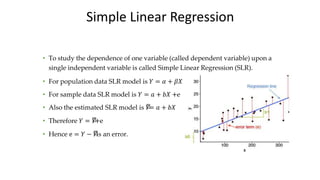
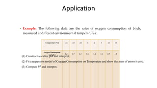
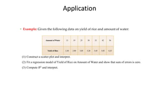
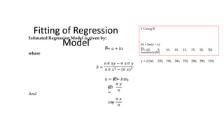
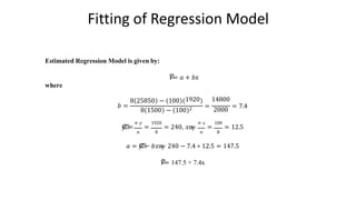
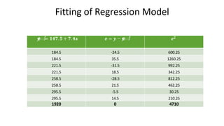
Here are the steps to estimate the relationship between VOL and HT for the given data: 1. Construct a scatter plot of VOL vs HT and interpret the relationship. 2. Fit a linear regression model of the form VOL = a + bHT and estimate the parameters a and b using least squares method. 3. Compute the coefficient of determination R2 and interpret the amount of variation in VOL explained by the linear relationship with HT. This will help estimate the potential lumber harvest (VOL) given the height (HT) of a forest stand.

1. REGRESSION ANALYSIS
PROF. DR. MUHAMMAD AZAM

2. Introduction
• The term regression was introduced by Sir Francis Galton in
connection with height of parents and their children. For this
purpose he collected heights data of 1000 parents and their
children. Finally he concluded that tall parents have tall children
and short parents have short children. But their children were not
as tall or short as their parents were i.e. their height tend towards
the average height. This tendency was called regression by
Galton.
• Today the term regression has quite different meanings. “It
investigates the dependence of one variable (dependent variable)
upon one or more other variables (called independent variables)
and provide an equation for estimating or predicting the average
value of dependent variable”.

3. Independent and Dependent Variable
• A variable whose value are fixed or
determined by an experimenter is called
Independent Variable e.g. amount of fertilizer
in different plots decided by the farmer. So
amount of fertilizer will be an independent
variable. It is also called regressor predictor.
• On the other hand a variable whose values are
influenced or affected by the values of an
independent variable is called dependent
variable e.g. wheat yield obtained from
different plots by using specified amount of
fertilizer.

4. Independent and Dependent
Variable

5. Simple Linear Regression
• To study the dependence of one variable (called dependent variable) upon a
single independent variable is called Simple Linear Regression (SLR).
• For population data SLR model is 𝑌 = 𝛼 + 𝛽𝑋 + 𝜀
• For sample data SLR model is 𝑌 = 𝑎 + 𝑏𝑋 +e
• Also the estimated SLR model is 𝑌
෠= 𝑎 + 𝑏𝑋
• Therefore 𝑌 = 𝑌
෠
+e
• Hence e = 𝑌 − 𝑌
෠
is an error.

6. Method of Least Squares
• Method of Least Squares: According to method of least squares, we obtain those
values of unknown parameters (𝛼, 𝛽 𝑒𝑡𝑐.) those will minimize the error sum of
squares i.e. this method provide us least or minimum value of σ 𝑒2 = σ 𝑌 − 𝑌
෠ 2
.
• Estimation of Parameters: The values of 𝛼 𝑎𝑛𝑑 𝛽 are estimated by using method
of least squares as:
𝑛 σ 𝑥2− σ 𝑥 2
• 𝑏 = 𝑛 σ 𝑥𝑦−σ 𝑥 σ 𝑦
and 𝑎 = 𝑦
ത
− 𝑏𝑥ҧ
• 𝑅2 = 1 −
σ 𝑒2
σ 𝑦
−
𝑦
ത 2
where σ 𝑦 − 𝑦
ത2 = 𝑛 σ 𝑦2 − σ 𝑦 2

7. Definitions
• Intercept: It is the value of dependent
variable without any influence of
independent variable. It is denoted by
“𝑎” which is an estimate of 𝛼.
• Regression Coefficient: It is the
change in the value of dependent
variable (Y) due to unite change in the
value of independent variable. It is
denoted by 𝑏 which is an estimate of
𝛽.

8. Application
• Example: The marketing manager of a large supermarket chain would like to use
shelf space to predict the sales of pet food. A random sample of 8 equal sized
stores is selected with the following results:
Shelf Space (Feet) 𝑥 5 5 10 10 15 15 20 20
Weekly Sales ($) 𝑦 160 220 190 240 230 280 290 310
(1) Construct a scatter plot and interpret.
(2) Fit a regression model of weekly sales on shelf space and show that sum of errors is zero.
(3) Compute 𝑅2 and interpret.

9. Scatter
Plot
X Y
5 160
5 220
10 190
10 240
15 230
15 280
20 290
20 310
10, 10, 15, 15, 20, 20)
x = c(5, 5,
y = c(160, 220, 190, 240, 230, 280, 290, 310)
plot(x, y, col = 2, main = "Scatter Plot", cex = 1.5, pch = 11)
# cex: character expansion
# pch: plot character

10. Fitting of Regression
Model
Estimated Regression Model is given by:
𝑌
෠= 𝑎 + 𝑏𝑥
where
𝑛 σ 𝑥𝑦 − σ 𝑥 σ 𝑦
𝑏 =
𝑛 σ 𝑥2 − σ 𝑥 2
𝑦
ത
=
𝑎 = 𝑦
ത
− 𝑏𝑥ҧ
σ 𝑦
𝑛
And
𝑥ҧ
=
σ 𝑥
𝑛
# Using R
x = c(5, 5, 10, 10, 15, 15, 20, 20)
y = c(160, 220, 190, 240, 230, 280, 290, 310)
fit = lm(y ~ x)
fit
summary(fit)

11. Fitting of Regression Model
x y x y x2 𝒚𝟐
5 160 800 25 25600
5 220 1100 25 48400
10 190 1900 100 36100
10 240 2400 100 57600
15 230 3450 225 52900
15 280 4200 225 78400
20 290 5800 400 84100
20 310 6200 400 96100
100 1920 25850 1500 479200

12. Fitting of Regression Model
Estimated Regression Model is given by:
𝑌
෠= 𝑎 + 𝑏𝑥
where
𝑏 =
8 25850 − 100
8 1500 − 100 2
1920 14800
=
2000
= 7.4
σ 𝑦 1920 σ 𝑥 100
𝑦
ത= = = 240, 𝑥ҧ
= = = 12.5
𝑛 8 𝑛 8
𝑎 = 𝑦
ത
− 𝑏𝑥ҧ
= 240 − 7.4 ∗ 12.5 = 147.5
𝑌
෠= 147.5 + 7.4x

13. Fitting of Regression Model
𝒚
ෝ = 𝟏𝟒𝟕. 𝟓 + 𝟕. 𝟒𝒙 𝒆 = 𝒚 − 𝒚
ෝ 𝒆𝟐
184.5 -24.5 600.25
184.5 35.5 1260.25
221.5 -31.5 992.25
221.5 18.5 342.25
258.5 -28.5 812.25
258.5 21.5 462.25
295.5 -5.5 30.25
295.5 14.5 210.25
1920 0 4710

14. Coefficient of Determination (𝑅2)
𝑅2 = 1 −
σ 𝑒2
σ 𝑦
−
𝑦
ത 2
where σ 𝑦 − 𝑦
ത2 = σ 𝑦2 −
σ 𝑦 2
𝑛
෠ 𝑦 − 𝑦
ത2 = ෠ 𝑦2 −
σ 𝑦 2
𝑛
8
2
σ 𝑦 − 𝑦
ത2 = 479200 − 1920
= 18400
𝑅2 = 1 −
4710
18400
= 0.7440 or 74.40%
It mean contribution of Shelf Space (in feet) is 74.40% in Weekly Sales (in $) of pet
food.

15. Coefficient of Determination (𝑅2)
about the
It is the ratio between “Explained Variation” and “Total Variation”. It tells us
contribution of independent variable into the dependent variable. Here
Total Variation = Explained Variation + Unexplained Variation
Explained Variation = Total Variation – Unexplained Variation
𝑅2 =
𝐸𝑥𝑝𝑙𝑎𝑖𝑛𝑒𝑑 𝑉𝑎𝑟𝑖𝑎𝑡𝑖𝑜𝑛
=
Total Variation – Unexplained Variation
𝑇𝑜𝑡𝑎𝑙 𝑉𝑎𝑟𝑖𝑎𝑡𝑖𝑜𝑛 Total Variation
𝑅2 = 1 − = 1 −
Unexplained Variation σ 𝑒2
Total Variation σ 𝑦 − 𝑦
ത2
Where σ 𝑒2 = σ 𝑦2 − 𝑎 σ 𝑦 − 𝑏 σ 𝑥𝑦
2
෠ 𝑦 − 𝑦
ത2 = 𝑛 ෠ 𝑦2 − ෠ 𝑦

16. Coefficient of Determination (𝑅2)
where 0 ≤ 𝑅2 ≤ 1 and is usually expressed in percentage. For Example: 𝑅2 =
0.85 or 85%; it means contribution of independent variable is 85% into the total
variation in dependent variable. In other word 85% of the variation in dependent
variable is due to independent variable.

17. Application
• Example: The following data are the rates of oxygen consumption of birds,
measured at different environmental temperatures:
Temperature (oC) -18 -15 -10 -5 0 5 10 19
Oxygen Consumption
(ml/g/hr) 5.2 4.7 4.5 3.6 3.4 3.1 2.7 1.8
(1) Construct a scatter plot and interpret.
(2) Fit a regression model of Oxygen Consumption on Temperature and show that sum of errors is zero.
(3) Compute 𝑅2 and interpret.

18. Application
• Example: Given the following data on yield of rice and amount of water:
Amount of Water 13 19 25 30 33 42 56
Yield of Rice 2.30 2.90 3.05 3.20 3.45 3.85 4.25
(1) Construct a scatter plot and interpret.
(2) Fit a regression model of Yield of Rice on Amount of Water and show that sum of errors is zero.
(3) Compute 𝑅2 and interpret.

19. Application
• Example: One task is assigned to foresters is to estimate the
potential lumber harvest of a forest. The description of variables
is as under: HT: the height in feet and VOL: the volume of
lumber (a measure of the yield) in cubic feet.
• HT: 89.00, 90.07, 95.08, 98.03, 99.00, 91.05, 105.60, 100.80,
94.00, 93.09
• VOL: 25.93, 45.87, 56.20, 58.60, 63.36, 46.35, 68.99, 62.91,
58.13, 59.79
• Estimate the relationship betweenVOL andHT for