1. Automatic Calibration of a Three-Axis Magnetic
Compass
Raj Sodhi
Wednesday, June 1, 2005
PNI's family of tilt compensated magnetic compasses, or TCM modules,
are beginning to show widespread acceptance in the marketplace. The
automatic calibration algorithm we shall describe allows the TCM to
characterize its magnetic environment while the user rotates the unit
through various orientations. This algorithm must also characterize and
correct for a residual rotation between the magnetometer and
accelerometer coordinate systems. This is an extremely difficult task,
especially considering that the module will often be used in a noisy
environment, and many times will not be given the full range of rotations
possible during the calibration. Given a successful user calibration with its
underlying factory calibration s, heading accuracies of 2° or better may
be of achieved, even under severe pitch and roll conditions.
First, we shall introduce the concepts of soft and hard iron distortion,
providing a little mathematical background. Then, we shall present the
two stages of the algorithm, along with the procedure for recursive least
squares. Finally, we shall present the results of a simulation putting all
these to use.
Magnetic Distortion Introduction
For the magnetometers to be perfectly calibrated for magnetic
compassing, they must only sense Earth's magnetic field, and nothing else.
With an ideal triaxial magnetometer, the measurements will seem to ride
along the surface of a sphere of constant radius, which we may call our
"measurement space.” The end-user may install a perfectly calibrated
module from the factory into an application whose magnetic
environment leads to distortions of this measurement space, and
therefore a significant degradation in heading accuracy. The two most
common impairments to the measurement space are hard and soft iron
distortion. Hard iron distortion may be described as a fixed offset bias to
the readings, effectively shifting the origin of our ideal measurement
space. It may be caused by a permanent magnet mounted on or
around the fixture of the compass installation. Soft iron distortion is a
direction dependent distortion of the gains of the magnetometers, often
caused by the presence of high permeability materials in or around the
compass fixture. Figure 1 shows the unimpaired measurement space, or
the locus of measurements for a perfectly calibrated magnetometer.

2. Figure 2 shows the magnetometer with a hard iron distortion impairment
of 10 uT in the X direction, 20 uT in the Y direction, and 30 uT in the Z
direction, and soft iron distortion impairments. One may observe that the
locus of measurements has now changed from being spherical to
ellipsoidal.
Figure 1. Measurement space for perfectly calibrated magnetometer
without hard iron and soft iron distortions.
Figure 2. Measurement space with hard and soft iron distortions.
We will represent the undistorted Earth's magnetic field as “Be”, and what
is measured as “Bm”. To go from one to the other, we may use the
following equations.

3. −1
(eq. 1) Bm S ⋅ Be + H Be S⋅ ( Bm − H)
The soft iron matrix “S” is 3 x 3, and the hard iron vector “H” is 3 x 1. It will
be our job to undo the effects of S and H in terms of heading accuracy.
Algorithm Derivation
From the three magnetometers and three accelerometers, we receive six
streams of data. At regular intervals of roughly 30 ms, we put the readings
from each sensor together to approximately take a snapshot of the
modules orientation. We say "approximately" here because there is
indeed a delay between when the X magnetometer has been queried
and when the Z magnetometer has been queried. Assuming that we
have an ideal module that can make error-free measurements of the
local magnetic field and acceleration instantly, we may make the
following two very important statements.
• The magnitude of Earth's magnetic field is constant, regardless the
TCM's orientation.
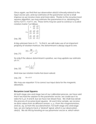
• The angle formed between Earth's magnetic field vector and Earth's
gravitational acceleration vector is constant, once again regardless
the TCM's orientation.
The algorithm is founded on the above two statements. We use the first
statement to mathematically bend and stretch the magnetometer axes
such that they are orthogonal to each other and gain matched. At this
stage, we also determine the hard iron offset vectors. We use the second
statement to determine a rotation matrix that may be used to fine tune
our estimate of the soft iron distortion, and to align the magnetometer
coordinate system with the accelerometer coordinate system. Therefore,
the algorithm comes in two stages. The first stage centers our ellipsoidal
measurement space about the origin, and makes it spherical. The second
stage rotates the sphere slightly.
We may express the magnitude of Earth's magnetic field in terms of our
measurement vector Bm.
(eq. 2) ( Be )2 T
[ [ S⋅ ( Bm − H) ] ] ⋅ [ S⋅ ( Bm − H) ] (BmT − HT)⋅ST⋅S⋅(Bm − H)
The middle term may be expressed as a single 3 x 3 symmetrical matrix, C.
T
(eq. 3) C S S
Multiplying these terms out, we get the following quadratic equation.

4. (eq. 4) ( Be )2 T T
Bm C⋅ Bm − 2⋅ Bm C⋅ H + H C⋅ H
T
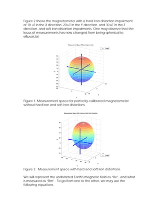
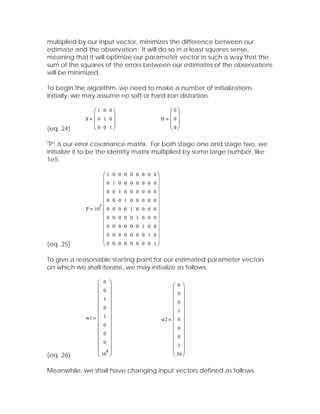
Stage One of Calibration Process
At this stage, we shall assume that our soft iron matrix is upper triangular,
correcting for this assumption in the second stage of the calibration.
(eq. 5)
⎛ 1 s12 s13 ⎞
⎛ 1 0 0 ⎞ ⎛ 1 s12 s13 ⎞ ⎜ ⎟
T ⎜ s12 s22 0 ⎟ ⋅ ⎜ 0 s22 s23 ⎟ 2 2
S_ut S_ut ⎜ s12 s12 + s22 s12⋅ s13 + s22⋅ s23 ⎟
⎜ ⎟⎜ ⎟
⎝ s13 s23 s33 ⎠ ⎝ 0 0 s33 ⎠ ⎜ 2 2 2⎟
⎝ s13 s12⋅ s13 + s22⋅ s23 s13 + s23 + s33 ⎠
⎛ 1 c12 c13 ⎞
C S_ut S_ut
T ⎜ c12 c22 c23 ⎟
⎜ ⎟
(eq. 6) ⎝ c13 c23 c33 ⎠
If we assume that our measurement Bm may be expressed as a 3 x 1
vector of [x, y, z]T, we obtain the following.
⎛ 1 c12 c13 ⎞ ⎛ x ⎞
( x y z ) ⋅ ⎜ c12 c22 c23 ⎟ ⋅ ⎜ y ⎟ − 2⋅ ( x y z ) ⋅ C⋅ H + H ⋅ C⋅ H ( Be )
T 2
⎜ ⎟⎜ ⎟
(eq. 7) ⎝ c13 c23 c33 ⎠ ⎝ z ⎠
There are three parts to this equation. We shall deal with each separately.
The first part may be expanded to give terms that are second-order.
2 2 2
(eq. 8) T1 x + 2⋅ x⋅ y ⋅ c12 + 2⋅ x⋅ z⋅ c13 + y ⋅ c22 + 2⋅ y ⋅ z⋅ c23 + z ⋅ c33
The second gives rise to terms that are linear with respect to x, y and z.
⎛ Lx ⎞
T2 −2⋅ ( x y z ) ⋅ C⋅ H −2⋅ ( x y z ) ⋅ ⎜ Ly ⎟ −2⋅ x⋅ Lx − 2⋅ y ⋅ Ly − 2⋅ z⋅ Lz
⎜ ⎟
(eq. 9) ⎝ Lz ⎠
The constant terms may be grouped as follows.
(eq. 10) T3
T
H ⋅ C⋅ H − ( Be )2

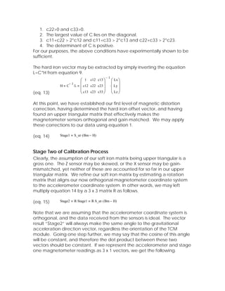
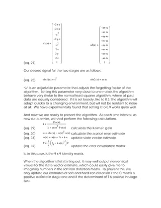
5. After some algebraic manipulations, we may recast this equation as the
inner product of two vectors: a changing input vector, and our estimation
parameter vector.
T
⎛ −2⋅ x⋅ y ⎞
⎜ ⎟ ⎡ c12 ⎤
⎜ −2⋅ x⋅ z ⎟ ⎢ c13
⎥
⎜ 2 ⎟ ⎢ ⎥
⎜ −y ⎟ ⎢ c22 ⎥
⎜ −2⋅ y ⋅ z ⎟ ⎢ c23 ⎥
⎢ ⎥
u(n) ⋅ w ⎜ ⎟
2 T
obs ( n ) x 2 ⋅⎢ c33 ⎥
⎜ −z ⎟ ⎢ ⎥
Lx
⎜ 2⋅ x ⎟ ⎢ ⎥
⎜ ⎟ ⎢
Ly
⎥
⎜ 2⋅ y ⎟ ⎢ Lz ⎥
⎜ 2⋅ z ⎟
⎜ 1 ⎟ ⎢ T 2⎥
(eq. 11) ⎝ ⎠ ⎣H ⋅ C⋅ H − ( Be ) ⎦
Since our observation obs(n) and the input vector u(n) are linearly related
by w, we may continue to make improvements on our estimates of w as
these data are streaming by. Let us assume that using recursive least
squares, we have obtained good estimates of the parameters c12, c13,
c22, c23, c33, Lx, Ly and Lz. First we organize our the first five parameters
into the C matrix as defined in equation 6. Then we may extract our upper
triangular soft iron matrix by taking the Cholesky decomposition. The
Cholesky decomposition may be thought of as taking the square root of a
matrix. If a square matrix is “positive definite” (which we will define
shortly), then we may factor this matrix into the product of UT*U, where U is
upper triangular, and UT is lower triangular. Applying this concept to our C
matrix...
⎛ ⎛ 1 c12 c13 ⎞ ⎞ ⎛ 1 s12 s13 ⎞
S_ut chol ( C) chol ⎜ ⎜ c12 c22 c23 ⎟ ⎟ ⎜ 0 s22 s23 ⎟
⎜⎜ ⎟⎟ ⎜ ⎟
(eq. 12) ⎝ ⎝ c13 c23 c33 ⎠ ⎠ ⎝ 0 0 s33 ⎠
However, we cannot take the Cholesky decomposition of any matrix. As
we are iteratively improving our estimates of the parameters in w, we may
well stumble upon a C matrix where the Cholesky decomposition fails. To
guarantee the success of this operation, we must test to see if the C matrix
is positive definite. Strictly speaking, a positive definite matrix A may be
pre-multiplied and post-multiplied by any vector x to give rise to a positive
scalar constant. xT*A*x > 0. But this is not very useful, as we do not have
time to test this condition on hundreds upon thousands of test vectors.
Fortunately, there is an easier way. The following are necessary but not
sufficient conditions on our C matrix to be positive definite. [1]

6. 1. c22>0 and c33>0.
2. The largest value of C lies on the diagonal.
3. c11+c22 > 2*c12 and c11+c33 > 2*c13 and c22+c33 > 2*c23.
4. The determinant of C is positive.
For our purposes, the above conditions have experimentally shown to be
sufficient.
The hard iron vector may be extracted by simply inverting the equation
L=C*H from equation 9.
−1
⎛ 1 c12 c13 ⎞ ⎛ Lx ⎞
H C ⋅ L ⎜ c12 c22 c23 ⎟ ⋅ ⎜ Ly ⎟
−1
⎜ ⎟ ⎜ ⎟
(eq. 13) ⎝ c13 c23 c33 ⎠ ⎝ Lz ⎠
At this point, we have established our first level of magnetic distortion
correction, having determined the hard iron offset vector, and having
found an upper triangular matrix that effectively makes the
magnetometer sensors orthogonal and gain matched. We may apply
these corrections to our data using equation 1.
(eq. 14) Stage1 S_ut ⋅ ( Bm − H)
Stage Two of Calibration Process
Clearly, the assumption of our soft iron matrix being upper triangular is a
gross one. The Z sensor may be skewed, or the X sensor may be gain-
mismatched, yet neither of these are accounted for so far in our upper
triangular matrix. We refine our soft iron matrix by estimating a rotation
matrix that aligns our now orthogonal magnetometer coordinate system
to the accelerometer coordinate system. In other words, we may left
multiply equation 14 by a 3 x 3 matrix R as follows.
(eq. 15) Stage2 R⋅ Stage1 R⋅ S_ut ⋅ ( Bm − H)
Note that we are assuming that the accelerometer coordinate system is
orthogonal, and the data received from the sensors is ideal. The vector
result “Stage2” will always make the same angle to the gravitational
acceleration direction vector, regardless the orientation of the TCM
module. Going one step further, we may say that the cosine of this angle
will be constant, and therefore the dot product between these two
vectors should be constant. If we represent the accelerometer and stage
one magnetometer readings as 3 x 1 vectors, we get the following.

7. ⎛ ax ⎞ ⎛ r11 r12 r13 ⎞ ⎛ xc ⎞
Accel ⎜ ay ⎟ Mag R⋅ Stage1 ⎜ r21 r22 r23 ⎟ ⋅ ⎜ yc ⎟
⎜ ⎟ ⎜ ⎟⎜ ⎟
(eq. 16) ⎝ az ⎠ and ⎝ r31 r32 r33 ⎠ ⎝ zc ⎠
The dot product may be expressed as follows.
⎛ r11 r12 r13 ⎞ ⎛ xc ⎞
( ax ay az ) ⋅ ⎜ r21 r22 r23 ⎟ ⋅ ⎜ yc ⎟
T
Accel ⋅ Mag constant
⎜ ⎟⎜ ⎟
(eq. 17) ⎝ r31 r32 r33 ⎠ ⎝ zc ⎠
Dividing through by r11,
⎛ r12 r13 ⎞
⎜ 1
r11 r11 ⎟
⎜ ⎟ ⎛ xc ⎞
( ax ay az ) ⋅ ⎜
r21 r22 r23 ⎟
⋅ ⎜ yc ⎟
constant
⎜ r11 r11 r11 ⎟ ⎜ ⎟ r11
⎜ ⎝ zc ⎠
r31 r32 r33 ⎟
⎜ ⎟
(eq. 18) ⎝ r11 r11 r11 ⎠
As we had done in stage one (equation 11), we may cast our linear
equation as the inner product of an input vector and a parameter vector.
⎛ r12 ⎞
⎜ r11 ⎟
⎜ ⎟
⎜ r13 ⎟
⎜ r11 ⎟
T
⎜ r21 ⎟
⎛ −ax⋅ yc ⎞ ⎜
⎜ ⎟ ⎜
⎟
r11
⎟
⎜ −ax⋅ zc ⎟ ⎜ r22 ⎟
⎜ −ay ⋅ xc ⎟ ⎜ ⎟
⎜ ⎟ ⎜ r11
⎟
−ay ⋅ yc
⎜ ⎟
obs ( n ) ax⋅ xc u ( n ) ⋅ w ⎜ −ay ⋅ zc ⎟ ⋅ ⎜ ⎟
T r23
⎜ r11 ⎟
⎜ −az⋅ xc ⎟ ⎜ ⎟
⎜ ⎟ r31
⎜ −az⋅ yc ⎟ ⎜ r11
⎟
⎜ ⎟
⎜ −az⋅ zc ⎟ ⎜ r32 ⎟
⎜ 1 ⎟ ⎜
⎝ ⎠ ⎟
r11
⎜ r33
⎟
⎜ ⎟
⎜ r11 ⎟
⎜ T ⎟
⎜ −Accel ⋅ Mag ⎟
(eq. 19) ⎝ r11 ⎠

8. Once again, we find that our observation obs(n) is linearly related to the
input vector u(n), and our estimates of the parameter vector w shall
improve as we receive more and more data. Thanks to the recursive least
squares algorithm, we may estimate the parameters in w, obtaining the
terms r12/r11, r13/r11, etc. These terms may be used to construct a scaled
rotation matrix T as follows.
⎛ 1 r12 r13 ⎞
⎜ r11 r11 ⎟
⎜ ⎟
T ⎜ r21 r22 r23 ⎟
⎜ r11 r11 r11 ⎟
⎜ r31 r32 r33 ⎟
⎜ ⎟
(eq. 20) ⎝ r11 r11 r11 ⎠
A big unknown here is r11. To find it, we will make use of an important
property of rotation matrices: the determinant is always equal to one.
R 1
T
3 3
(eq. 21) r11 r11
So only if the above determinant is positive, we may update our estimate
of r11.
1
3
⎛ 1 ⎞
r11 ⎜ T ⎟
(eq. 22) ⎝ ⎠
And now our rotation matrix has been solved.
(eq. 23) R r11⋅ T
We may use equation 15 to correct our input data for the magnetic
distortions.
Recursive Least Squares
At both stage one and stage two of our calibration process, we have said
that if we had the solution to the parameter vector, we could use it to
solve for S_ut, H and R, but we have not shown how. We shall now detail
the process of recursive least squares. At each time sample, we receive
six data values from six different sensors: x, y, z from the magnetometers,
and ax, ay, az from the accelerometers. For both stage one and stage
two, we are trying to track a "desired" signal, which is our observation,
obs(n). We do this by iterating on our parameter vector w, which when

9. multiplied by our input vector, minimizes the difference between our
estimate and the observation. It will do so in a least squares sense,
meaning that it will optimize our parameter vector in such a way that the
sum of the squares of the errors between our estimates of the observations
will be minimized.
To begin the algorithm, we need to make a number of initializations.
Initially, we may assume no soft or hard iron distortion.
⎛1 0 0⎞ ⎛0⎞
S ⎜0 1 0⎟ H ⎜0⎟
⎜ ⎟ ⎜ ⎟
(eq. 24) ⎝0 0 1⎠ ⎝0⎠
"P” is our error covariance matrix. For both stage one and stage two, we
initialize it to be the identity matrix multiplied by some large number, like
1e5.
⎛1
⎜
0 0 0 0 0 0 0 0⎞
⎟
⎜0 1 0 0 0 0 0 0 0⎟
⎜0 0 1 0 0 0 0 0 0⎟
⎜ ⎟
5
⎜0 0 0 1 0 0 0 0 0
⎟
P 10 ⋅ ⎜ 0 0 0 0 1 0 0 0 0⎟
⎜0 0 0 0 0 1 0 0 0⎟
⎜ ⎟
⎜0 0 0 0 0 0 1 0 0⎟
⎜0 0 0 0 0 0 0 1 0⎟
⎜0 1⎟
(eq. 25) ⎝ 0 0 0 0 0 0 0 ⎠
To give a reasonable starting point for our estimated parameter vectors
on which we shall iterate, we may initialize as follows.
⎛ 0 ⎞ ⎛0⎞
⎜ 0 ⎟ ⎜ ⎟
⎜ ⎟ ⎜0⎟
⎜ 1 ⎟ ⎜0⎟
⎜ 0 ⎟ ⎜1⎟
⎜ ⎟ ⎜ ⎟
w1 ⎜ 1 ⎟ w2 ⎜ 0 ⎟
⎜ 0 ⎟ ⎜0⎟
⎜ 0 ⎟ ⎜ ⎟
⎜ ⎟ ⎜0⎟
⎜ 0 ⎟ ⎜1⎟
⎜ 4⎟ ⎜ 50 ⎟
(eq. 26) ⎝ 10 ⎠ ⎝ ⎠
Meanwhile, we shall have changing input vectors defined as follows.

10. ⎛ −2⋅ x⋅ y ⎞
⎜ ⎟
⎜ −2⋅ x⋅ z ⎟ ⎛ −ax⋅ yc ⎞
⎜ ⎟
⎜ 2 ⎟ ⎜ −ax⋅ zc ⎟
⎜ −y ⎟ ⎜ −ay ⋅ xc ⎟
⎜ −2⋅ y⋅ z ⎟ ⎜ ⎟
u1( n ) ⎜ 2
⎟ ⎜ −ay ⋅ yc ⎟
⎜ −z ⎟ u2( n ) ⎜ −ay ⋅ zc ⎟
⎜ 2⋅ x ⎟ ⎜ −az⋅ xc ⎟
⎜ ⎟ ⎜ ⎟
⎜ 2⋅ y ⎟ ⎜ −az⋅ yc ⎟
⎜ 2⋅ z ⎟ ⎜ −az⋅ zc ⎟
⎜ 1 ⎟ ⎜ 1 ⎟
(eq. 27) ⎝ ⎠ ⎝ ⎠
Our desired signal for the two stages are as follows.
2
(eq. 28) obs1 ( n ) x obs2 ( n ) ax⋅ xc
“λ” is an adjustable parameter that adjusts the forgetting factor of the
algorithm. Setting this parameter very close to one makes the algorithm
behave very similar to the normal least squares algorithm, where all past
data are equally considered. If it is set loosely, like to 0.5, the algorithm will
adapt quickly to a changing environment, but will not be resistant to noise
at all. We have experimentally found that setting it to 0.9 works quite well.
And now we are ready to present the algorithm. At each time interval, as
new data arrives, we shall perform the following calculations.
P⋅ u ( n )
k
T
(eq. 29) λ + u ( n ) ⋅ P⋅ u ( n ) calculate the Kalman gain
T
(eq. 30) α obs ( n ) − w( n ) ⋅ u ( n ) calculate the a priori error estimate
(eq. 31) w( n ) w( n − 1) + k⋅ α update state vector estimate
⋅ ⎛ I − k⋅ u ( n )
1 T⎞
P ⋅P
(eq. 32) λ ⎝ 9 ⎠ update the error covariance matrix
I9, in this case, is the 9 x 9 identity matrix.
When the algorithm is first starting out, it may well output nonsensical
values for the state vector estimate, which could easily give rise to
imaginary numbers in the soft iron distortion matrix. To prevent this, we
only update our estimates of soft and hard iron distortion if the C matrix is
positive definite in stage one and if the determinant of T is positive in stage
two.

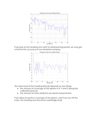
11. Algorithm Simulation
The algorithm described above was implemented in Matlab. In San
Francisco, the magnitude of Earth's magnetic field is 49.338 uT, the dip
angle is 61.292°, and the declination is 14.814°. This means that the X, Y
and Z components of Earth's magnetic field are [22.9116 ; 6.0595 ; 43.2733]
uT. The gravitational acceleration may be represented by [0 ; 0 ; 1]. We
assume that there are 100 samples submitted to the algorithm. We
randomize the yaw, pitch and roll so that they vary between 0 - 360°, 25 -
65°, and -40 – 40° respectively.
For each triad of yaw, pitch and roll, a 3 x 3 rotation matrix is calculated to
move from our Earth inertial reference frame coordinate system to that of
the compass. Once the transformation matrix has been calculated, it
may be used to multiply the North vector and the gravity vector to
simulate our ideal measurements.
The soft iron distortion matrix was randomly generated, and yet designed
to be close to the identity matrix.

12. Actual SI = [
0.9567 0.0288 0.1189
-0.1666 0.8854 -0.0038
0.0125 0.1191 1.0327
];
The hard iron vector was chosen as [ 10 ; 20 ; 30 ] uT.
These magnetic distortion impairments were applied to the data to
simulate our measured data. To make this data seem more real, 30 nT
RMS noise was added to the magnetometer data and 3 mG RMS noise
was added to the accelerometer data. Finally, the data were submitted
to the recursive least squares estimation algorithm. Initially, the algorithm
did very poorly with regards to heading accuracy. But as the algorithm
learned about its magnetic impairments, the heading error diminished.

13. If we look at the heading error after its initial learning period, we may get
a feel for the accuracy of our simulated compass.
The noise level of the heading directly depends on two things.
• the amount of coverage of the sphere in X, Y and Z during the
calibration process.
• the amount of noise added to our ideal measurements.
If we allow for perfect coverage of the sphere, and if we turn off the
noise, the heading error becomes vanishingly small.

14. Concluding Remarks
The three dimensional auto calibration algorithm presented above has
enormous potential for magnetic compassing applications such as in cell
phones, PDAs, etc. Based on how much noise is added to the raw
measurements, and based on how much of the sphere has been covered
over the course of the algorithm, we may see heading errors of 2° or less.
References.
[1]. http://mathworld.wolfram.com/PositiveDefiniteMatrix.html
[2]. Haykin, Simon, Adaptive Filter Theory, third edition, Prentice-Hall, 1996,
chapters 11 and 13.
[3]. Lecture Notes by Professor Ioan Tabus at
http://www.cs.tut.fi/~tabus/course/ASP/Lectures_ASP.html