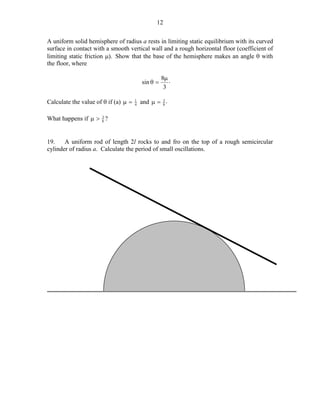
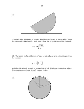
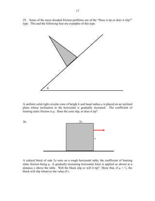
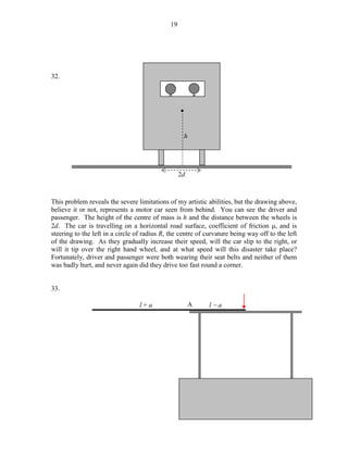
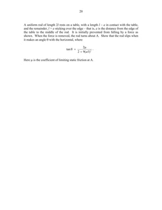
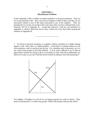
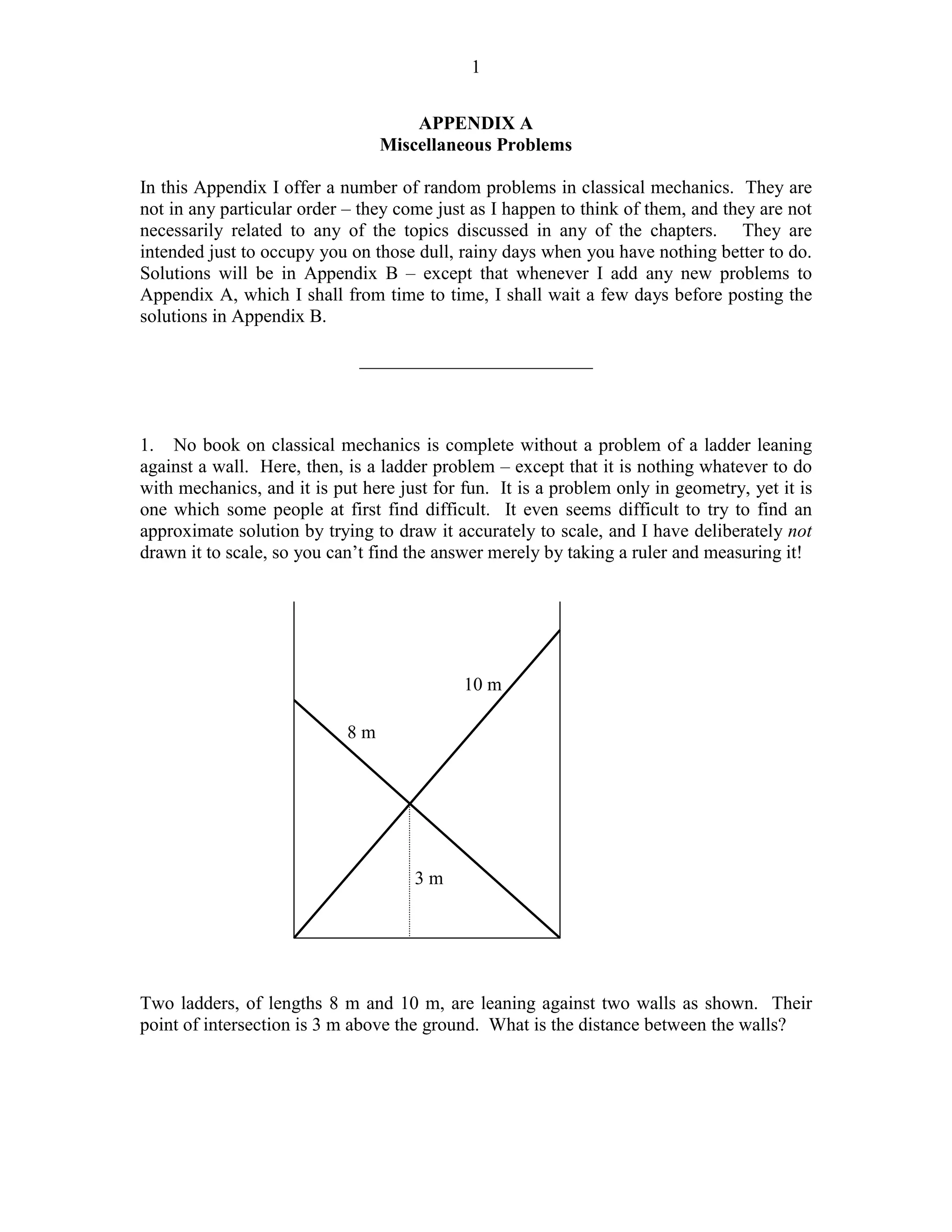
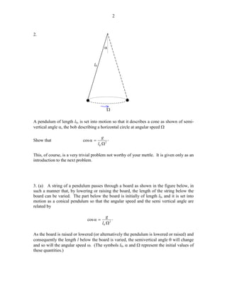
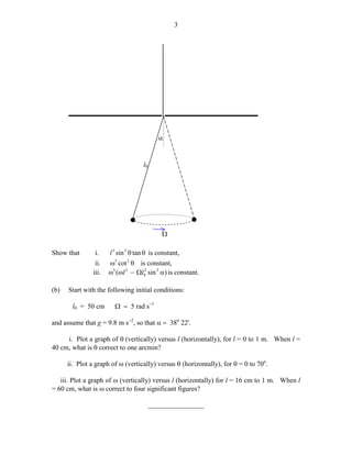
The document contains 14 problems related to classical mechanics. Problem 1 describes two ladders leaning against two walls, with their intersection point 3 m above the ground, and asks for the distance between the walls. Problem 3 involves a pendulum whose length below a board can be varied, and asks the reader to show various relationships involving the semi-vertical angle, angular speed, and pendulum length are constant. Problem 4 describes a rod initially vertical on a table that is given an angular displacement and falls over, and asks for expressions involving the rod's angular speed, center speed, lower end speed, and the table's normal reaction.

1. 1
APPENDIX A
Miscellaneous Problems
In this Appendix I offer a number of random problems in classical mechanics. They are
not in any particular order – they come just as I happen to think of them, and they are not
necessarily related to any of the topics discussed in any of the chapters. They are
intended just to occupy you on those dull, rainy days when you have nothing better to do.
Solutions will be in Appendix B – except that whenever I add any new problems to
Appendix A, which I shall from time to time, I shall wait a few days before posting the
solutions in Appendix B.
_________________________
1. No book on classical mechanics is complete without a problem of a ladder leaning
against a wall. Here, then, is a ladder problem – except that it is nothing whatever to do
with mechanics, and it is put here just for fun. It is a problem only in geometry, yet it is
one which some people at first find difficult. It even seems difficult to try to find an
approximate solution by trying to draw it accurately to scale, and I have deliberately not
drawn it to scale, so you can’t find the answer merely by taking a ruler and measuring it!
10 m
8m
3m
Two ladders, of lengths 8 m and 10 m, are leaning against two walls as shown. Their
point of intersection is 3 m above the ground. What is the distance between the walls?

2. 2
2.
α
l0
*
*
Ω
A pendulum of length l0, is set into motion so that it describes a cone as shown of semivertical angle α, the bob describing a horizontal circle at angular speed Ω
Show that
cos α =
g .
l0 Ω 2
This, of course, is a very trivial problem not worthy of your mettle. It is given only as an
introduction to the next problem.
3. (a) A string of a pendulum passes through a board as shown in the figure below, in
such a manner that, by lowering or raising the board, the length of the string below the
board can be varied. The part below the board is initially of length l0, and it is set into
motion as a conical pendulum so that the angular speed and the semi vertical angle are
related by
cos α =
g .
l0 Ω 2
As the board is raised or lowered (or alternatively the pendulum is lowered or raised) and
consequently the length l below the board is varied, the semivertical angle θ will change
and so will the angular speed ω. (The symbols l0, α and Ω represent the initial values of
these quantities.)

3. 3
α
l0
*
*
Ω
Show that
i.
ii.
iii.
(b)
l 3 sin 3 θ tan θ is constant,
ω3 cot 2 θ is constant,
ω3 (ωl 2 − Ωl02 sin 2 α ) is constant.
Start with the following initial conditions:
l0 = 50 cm
Ω = 5 rad s−1
and assume that g = 9.8 m s−2, so that α = 38o 22'.
i. Plot a graph of θ (vertically) versus l (horizontally), for l = 0 to 1 m. When l =
40 cm, what is θ correct to one arcmin?
ii. Plot a graph of ω (vertically) versus θ (horizontally), for θ = 0 to 70o.
iii. Plot a graph of ω (vertically) versus l (horizontally) for l = 16 cm to 1 m. When l
= 60 cm, what is ω correct to four significant figures?
________________

4. 4
The next few problems involve a rod with its lower end in contact with a horizontal table
and the rod falling over from an initial vertical (or inclined) position. There are several
versions of this problem. The table could be smooth, so that the rod freely slips over the
table. Or the lower end could be freely hinged at the table, so that the lower end does not
move as the rod falls over. Or the table might be rough, so that the rod might or might
not slip.
4. A uniform rod of mass m and length 2l is initially vertical with its lower end in contact
with a smooth horizontal table. It is given an infinitesimal angular displacement from its
initial position, so that it falls over. When the rod makes an angle θ with the vertical,
find:
The angular speed of the rod;
The speed at which the centre of the rod is falling;
The speed at which the lower end of the rod is moving;
The normal reaction of the table on the rod.
Show that the speed of the lower end is greatest when θ = 37o 50'.
If the length of the rod is 1 metre, and g = 9.8 m s−2, what is the angle θ when the speed
of the lower end is 1 m s−1?
5. A uniform rod is initially vertical with its lower end smoothly hinged to a horizontal
table. Show that, when the rod falls over, the reaction of the hinge upon the rod is
vertical when the rod makes an angle 48o 11' with the vertical, and is horizontal when the
rod makes an angle 70o 31' with the vertical.
6. A uniform rod of length 1 metre, with its lower end smoothly hinged to a horizontal
table, is initially held at rest making an angle of 40o with the vertical. It is then released.
If g = 9.8 m s−1, calculate its angular speed when it hits the table in a horizontal position
(easy) and how long it takes to get there (not so easy).
7.
A uniform rod is initially vertical with its lower end in contact with a rough
horizontal table, the coefficient of friction being µ.
Show that:
a. If µ < 0.3706, the lower end of the rod must slip before the rod makes an
angle θ with the vertical of 35o 05'.
b. If µ > 0.3706, the rod will not slip before θ = 51o 15', but it will certainly
slip before θ = 70o 31' .
If µ = 0.25, at what angle θ will the lower end slip? If µ = 0.75?

5. 5
8. It is time for another ladder problem. Most ladders in elementary mechanics problems
rest on a rough horizontal floor and lean against a smooth vertical wall. In this problem,
both floor and wall are smooth. The ladder starts making an angle of α with the vertical,
and then it is released. It immediately starts to slip, of course. After a while it will cease
contact with the smooth vertical wall. Show that, at the moment when the upper end of
the ladder loses contact with the wall, the angle θ that the ladder makes with the vertical
is given by cos θ = 2 cos α .
3
9. If you managed that one all right, this one, which is somewhat similar, should be
easy. Maybe.
A uniform solid semicylinder of radius a and mass m is placed with its curved surface
against a smooth vertical wall and a smooth horizontal floor, its base initially being
vertical.
It is then released. Find the reaction N1 of the floor on the semicylinder and the reaction
N2 of the wall on the semicylinder when its base makes an angle θ with the vertical.
Show that the semicylinder loses contact with the wall when θ = 90o, and that it then
continues to rotate until its base makes an angle of 39o 46' with the vertical before it
starts to fall back.
_________________________

6. 6
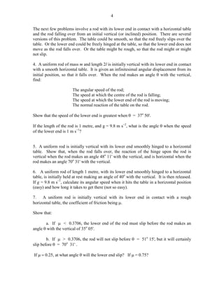
Many problems in elementary mechanics involve a body resting upon or sliding upon an
inclined plane. It is time to try a few of these. The first one is very easy, just to get us
started. The two following that might be more interesting.
10. A particle of mass m is placed on a plane which is inclined to the horizontal at an
angle α that is greater than tan −1 µ , where µ is the coefficient of limiting static friction.
What is the least force required to prevent the particle from sliding down the plane?
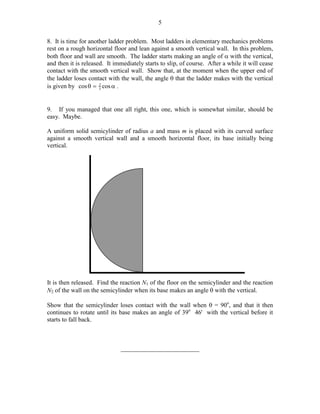
11. A cylinder or mass m, radius a, and rotational inertia ka2 rolls without slipping down
the rough hypotenuse of a wedge on mass M, the smooth base of which is in contact with
a smooth horizontal table. The hypotenuse makes an angle α with the horizontal, and the
gravitational acceleration is g. Find the linear acceleration of the wedge as it slips along
the surface of the table, in terms of m, M, g, a, k and α .
[Note that by saying that the rotational inertia is ka2, I am letting the question apply to a
hollow cylinder, or a solid cylinder, or even a hollow or solid sphere.]
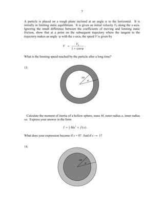
12.
x
V0
α
y

7. 7
A particle is placed on a rough plane inclined at an angle α to the horizontal. It is
initially in limiting static equilibrium. It is given an initial velocity V0 along the x-axis.
Ignoring the small difference between the coefficients of moving and limiting static
friction, show that at a point on the subsequent trajectory where the tangent to the
trajectory makes an angle ψ with the x-axis, the speed V is given by
V =
V0
.
1 + cos ψ
What is the limiting speed reached by the particle after a long time?
13.
xa
a
Calculate the moment of inertia of a hollow sphere, mass M, outer radius a, inner radius
xa. Express your answer in the form
2
I = 5 Ma 2 × f ( x) .
What does your expression become if x = 0? And if x → 1?
14.
xa
a

8. 8
Calculate the moment of inertia of a spherical planet of outer radius a, consisting of a
dense core of radius xa surrounded by a mantle of density s times the density of the core.
Express your answer in the form
2
I = 5 Ma 2 × f ( x , s ) .
Make sure that, if the density of the core is zero, your expression reduces to the answer
you got for problem 13.
2
Draw graphs of I / (5 Ma 2 ) versus x (x going from 0 to 1), for s = 0.2, 0.4, 0.6 and 0.8.
Show that, for a given mass M and density ratio s, the moment of inertia is least for a
core size give by the solution of
2(1 − s ) x 5 + 15 x 2 − 9 = 0 .
For a mantle-to-density ratio of 0.6, calculate the core size for which the moment of
inertia is least and calculate (in units of 2 Ma 2 ) the moment of inertia for that core.
5
Now let’s see if we can determine the core size from a knowledge of the moment of
inertia. It is sometimes asserted that one can determine the moment of inertia (and hence
the core size) of a planet from the rate of precession of the orbit of a satellite. I am not
sure how this would work with a planet such as Mercury, which has never had a satellite
in orbit around it. (Mariner 10, while in orbit around the Sun, made three fly-bys past
Mercury). Unless a planet departs from spherical symmetry, the orbit of a satellite will
not precess, since the gravitational planet is then identical with that from a point mass.
And, even if a planet were dynamically oblate, the rate of precession allows us to
determine the dynamical ellipticity (C − A)/C, but not either moment of inertia separately.
Nevertheless, let’s suppose that the moment of inertia of a planet is (0.92 ± 1%) %
2
2
5 Ma ; specifically, let’s suppose that the moment of inertia has been determined to be
between 0.911 and 0.929 % 2 Ma 2 , and that the mantle-to-core density ratio is known
5
(how?) to be 0.6. Calculate the possible range in the value of the core radius x.
15. A rectangular brick of length 2l rests (with the sides of length 2l vertically) on a
rough semicylindrical log of radius R. The drawing below shows three such bricks. In
the first one, 2l is quite short, and it looks is if it is stable. In the second one, 2l is rather
long, and the equilibrium looks decidedly wobbly. In the third one, we’re not quite sure
whether the equilibrium is stable or not. What is the longest brick that is stable against
small angular displacements from the vertical?

9. 9

10. 10
16. A Thing with a semicylindrical (or hemispherical) base of radius a is balanced on top
of a rough semicylinder (or hemisphere) of radius b as shown. The distance of the centre
of mass of the Thing from the line (or point) of contact is l. Show that the equilibrium is
stable if
1
1
1
>
+ .
l
a
b
*
l
a
b
If a = b, is the equilibrium stable if the Thing is
(1)
(2)
(3)
(4)
A hollow semicylinder?
A hollow hemisphere?
A uniform solid semicylinder?
A uniform solid hemisphere?

11. 11
17.
*
*
A log of square cross-section, sides 2a, rests on two smooth pegs a distance 2ac apart,
one of the diagonals making an angle θ with the vertical.
Show that, if c < 1 / 8 = 0.354 the only equilibrium position possible is θ = 90o, but
that this position is unstable; consequently, following a small displacement, the logs will
fall out of the pegs. Show that if the pegs are farther apart, with c > 0.354, three
equilibrium positions are possible. Which of them are stable, and which are unstable? If
c = 1 , what are the possible equilibrium values of θ?
2
18.
θ

12. 12
A uniform solid hemisphere of radius a rests in limiting static equilibrium with its curved
surface in contact with a smooth vertical wall and a rough horizontal floor (coefficient of
limiting static friction µ). Show that the base of the hemisphere makes an angle θ with
the floor, where
sin θ =
Calculate the value of θ if (a) µ =
1
4
8µ .
3
3
and µ = 8 .
3
What happens if µ > 8 ?
19.
A uniform rod of length 2l rocks to and fro on the top of a rough semicircular
cylinder of radius a. Calculate the period of small oscillations.

13. 13
20.
A uniform solid hemisphere of radius a with its curved surface in contact with a rough
horizontal table rocks through a small angle. Show that the period of small oscillations is
P = 2π
1.04a .
g
21. The density ρ of a solid sphere of mass M and radius a varies with distance r from
the centre as
r

ρ = ρ 0 1 −  .
a

Calculate the (second) moment of inertia about an axis through the centre of the sphere.
Express your answer in the form of constant % Ma2.
22.
*
α−θ
α+θ
*

14. 14
Two identical particles are connected by a light string of length 2aα. The system is
draped over a cylinder of radius a as shown, the coefficient of limiting static friction
being µ. Determine the angle θ when the system is in limiting equilibrium and just about
to slide.
F
23.
α
M
A mass M hangs from a light rope which passes over a rough cylinder, the coefficient of
friction being µ and the angle of lap being α. What is the least value of F, the tension in
the upper part of the rope, required to prevent the mass from falling?
24.
x
*
y

15. 15
A wooden cube floats on water. One of its faces is freely hinged to an axis fixed in the
surface of the water. The hinge is fixed at a distance from the top of the face equal to x
times the length of a side. The opposite face is submerged to a distance y times the
length of a side. Find the relative density s (that is, relative to the density of the water) of
the wood in terms of x and y.
25. A uniform solid sphere sits on top of a rough semicircular cylinder. It is given a
small displacement so that it rolls down the side of the cylinder. Show that the sphere
and cylinder part company when the line joining their centres makes an angle 53o 58'
with the vertical.
26.
12 cm
6 cm
9 cm

16. 16
A student has a triangular sandwich of sides 9 cm, 12 cm, 15 cm. She takes a
semicircular bite of radius 3 cm out of the middle of the hypotenuse. Where is the centre
of mass of the remainder? Is it inside or outside the bite?
27. An rubber elastic band is of length 2πa and mass m; the force constant of the rubber
is k. The band is thrown in the air, spinning, so that it takes the form of a circle, stretched
by the centrifugal force. (This takes much practice, skill and manual dexterity.) Find a
relation between its radius and angular speed, in terms of a, m and k.
28. Most of us have done simple problems on friction at high school or in first year at
college or university. You know the sort – a body lies on a rough horizontal table. A
force is applied to it. What happens? Try this one.
Find a uniform rod AB. A ruler will do as long as it is straight and not warped. Or a
pencil of hexagonal (not circular) cross-section, provided that it is uniform and doesn’t
have an eraser at the end. Place it on a rough horizontal table. Gradually apply a
horizontal force perpendicular to the rod at the end A until the rod starts to move. The
end A will, of course, move forward. Look at the end B – it moves backward. There is a
point C somewhere along the rod that is stationary. I.e., the initial motion of the rod is a
rotation about the point C. Calculate – and measure – the ratio AC/AB. What is the
force you are exerting on A when the rod is just about to move, in terms of its weight and
the coefficient of friction?

17. 17
29. Some of the more dreaded friction problems are of the “Does it tip or does it slip?”
type. This and the following four are examples of this type.
θ
A uniform solid right circular cone of height h and basal radius a is placed on an inclined
plane whose inclination to the horizontal is gradually increased. The coefficient of
limiting static friction is µ. Does the cone slip, or does it tip?
30.
2a
x
A cubical block of side 2a rests on a rough horizontal table, the coefficient of limiting
static friction being µ. A gradually increasing horizontal force is applied as shown at a
distance x above the table. Will the block slip or will it tip? Show that, if µ < ½, the
block will slip whatever the value of x.

18. 18
31.
τ
2ka
A cylindrical log of diameter 2a and mass m rests on two rough pegs (coefficient of
limiting static friction µ) a distance 2ka apart. A gradually increasing torque τ is applied
as shown. Does the log slip (i.e. rotate about its axis) or does it tip (about the right hand
peg)?
When you’ve done that one, you can try a variant (which I haven’t worked out and
haven’t posted a solution) in which a cylinder of radius a is resting against a kerb (or
curb, if you prefer that spelling) of height h, and a torque is applied. Will it tip or will is
slip?
h

19. 19
32.
•
h
2d
This problem reveals the severe limitations of my artistic abilities, but the drawing above,
believe it or not, represents a motor car seen from behind. You can see the driver and
passenger. The height of the centre of mass is h and the distance between the wheels is
2d. The car is travelling on a horizontal road surface, coefficient of friction µ, and is
steering to the left in a circle of radius R, the centre of curvature being way off to the left
of the drawing. As they gradually increase their speed, will the car slip to the right, or
will it tip over the right hand wheel, and at what speed will this disaster take place?
Fortunately, driver and passenger were both wearing their seat belts and neither of them
was badly hurt, and never again did they drive too fast round a corner.
33.
l+a
A
l−a

20. 20
A uniform rod of length 2l rests on a table, with a length l − a in contact with the table,
and the remainder, l + a sticking over the edge – that is, a is the distance from the edge of
the table to the middle of the rod. It is initially prevented from falling by a force as
shown. When the force is removed, the rod turns about A. Show that the rod slips when
it makes an angle θ with the horizontal, where
tan θ =
2µ
.
2 + 9(a/l ) 2
Here µ is the coefficient of limiting static friction at A.