Download as PDF, PPTX
![Given an array A with n elements, A[1…n]:
• DIVIDE (step 1)
Partition, i.e. re-arrange the elements of, array A[1…n] so that
for some element A[q]:
1. all elements on the left of A[q], i.e. A[1…q−1], are less than or
equal to A[q], and
2. all elements on the right of A[q], i.e. A[q+1…n], are greater
than or equal to A[q].
Quicksort divides & conquers](https://image.slidesharecdn.com/quicksort2019-190517113530/85/Quicksort-4-320.jpg)
![Given an array A with n elements, A[1…n]:
• DIVIDE (step 1)
Partition, i.e. re-arrange the elements of, array A[1…n] so that
for some element A[q]:
1. all elements on the left of A[q], i.e. A[1…q−1], are less than or
equal to A[q], and
2. all elements on the right of A[q], i.e. A[q+1…n], are greater
than or equal to A[q].
• CONQUER (step 2)
Sort sub-arrays A[1…q−1] and A[q+1…n] by recursive
executions of step 1.
Quicksort divides & conquers](https://image.slidesharecdn.com/quicksort2019-190517113530/85/Quicksort-5-320.jpg)
![Given an array A with n elements, A[1…n]:
• DIVIDE (step 1)
Partition, i.e. re-arrange the elements of, array A[1…n] so that
for some element A[q]:
1. all elements on the left of A[q], i.e. A[1…q−1], are less than or
equal to A[q], and
2. all elements on the right of A[q], i.e. A[q+1…n], are greater
than or equal to A[q].
• CONQUER (step 2)
Sort sub-arrays A[1…q−1] and A[q+1…n] by recursive
executions of step 1.
• COMBINE (step 3)
Just by joining the sorted sub-arrays we obtain a sorted array.
Quicksort divides & conquers](https://image.slidesharecdn.com/quicksort2019-190517113530/85/Quicksort-6-320.jpg)
![Given an array A with n elements, A[1…n]:
• DIVIDE (step 1)
Partition, i.e. re-arrange the elements of, array A[1…n] so that
for some element A[q]:
1. all elements on the left of A[q], i.e. A[1…q−1], are less than or
equal to A[q], and
2. all elements on the right of A[q], i.e. A[q+1…n], are greater
than or equal to A[q].
• CONQUER (step 2)
Sort sub-arrays A[1…q−1] and A[q+1…n] by recursive
executions of step 1.
• COMBINE (step 3)
Just by joining the sorted sub-arrays we obtain a sorted array.
Quicksort divides & conquers
Note:
• We will assume that the
elements of A are distinct.
• We will be sorting the elements
of A in an ascending order.](https://image.slidesharecdn.com/quicksort2019-190517113530/85/Quicksort-7-320.jpg)
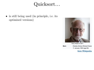
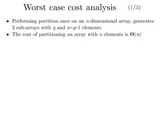
![Quicksort7.1 Description of quicksort
Combine: Because the subarrays are already
them: the entire array AŒp : : r is now sort
The following procedure implements quicksor
QUICKSORT.A; p; r/
1 if p < r
2 q D PARTITION.A; p; r/
3 QUICKSORT.A; p; q 1/
4 QUICKSORT.A; q C 1; r/
p r
… 6 5 1 … 22 9 2 …
}sub-array A[p…r]
both p, r are array indices](https://image.slidesharecdn.com/quicksort2019-190517113530/85/Quicksort-16-320.jpg)
![Quicksort
p q r
… 1 2 6 … 22 9 5 …
}sub-array A[p…r]
p, r, q are array indices
7.1 Description of quicksort
Combine: Because the subarrays are already
them: the entire array AŒp : : r is now sort
The following procedure implements quicksor
QUICKSORT.A; p; r/
1 if p < r
2 q D PARTITION.A; p; r/
3 QUICKSORT.A; p; q 1/
4 QUICKSORT.A; q C 1; r/](https://image.slidesharecdn.com/quicksort2019-190517113530/85/Quicksort-17-320.jpg)
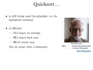
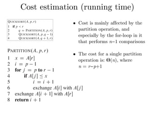
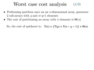
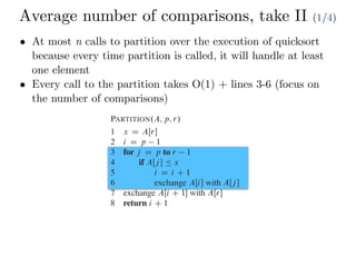
![Quicksort — Partition
2 q D PARTITION.A; p; r/
3 QUICKSORT.A; p; q 1/
4 QUICKSORT.A; q C 1; r/
To sort an entire array A, the initial call is QUICKSORT.A; 1; A:length/.
Partitioning the array
The key to the algorithm is the PARTITION procedure, which rearranges the su
ray AŒp : : r in place.
PARTITION.A; p; r/
1 x D AŒr
2 i D p 1
3 for j D p to r 1
4 if AŒj Ä x
5 i D i C 1
6 exchange AŒi with AŒj
7 exchange AŒi C 1 with AŒr
8 return i C 1
7.1 Description of quicksort
Combine: Because the subarrays are alr
them: the entire array AŒp : : r is no
The following procedure implements qu
QUICKSORT.A; p; r/
1 if p < r
2 q D PARTITION.A; p; r/
3 QUICKSORT.A; p; q 1/
4 QUICKSORT.A; q C 1; r/
To sort an entire array A, the initial call
Partition is the central sorting
operation of quicksort
p q? r
… 1 2 6 … 22 9 5 …
}sub-array A[p…r]
p, r, q are array indices](https://image.slidesharecdn.com/quicksort2019-190517113530/85/Quicksort-18-320.jpg)
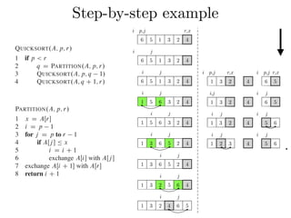
![Step-by-step exampleCombine: Because the subarrays are already sorted, no work is needed to combine
them: the entire array AŒp : : r is now sorted.
The following procedure implements quicksort:
QUICKSORT.A; p; r/
1 if p < r
2 q D PARTITION.A; p; r/
3 QUICKSORT.A; p; q 1/
4 QUICKSORT.A; q C 1; r/
To sort an entire array A, the initial call is QUICKSORT.A; 1; A:length/.
Partitioning the array
The key to the algorithm is the PARTITION procedure, which rearranges the subar-
ray AŒp : : r in place.
PARTITION.A; p; r/
1 x D AŒr
2 i D p 1
3 for j D p to r 1
4 if AŒj Ä x
5 i D i C 1
6 exchange AŒi with AŒj
7 exchange AŒi C 1 with AŒr
8 return i C 1
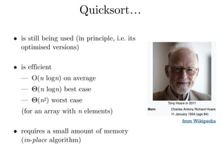
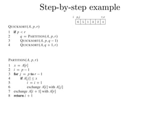
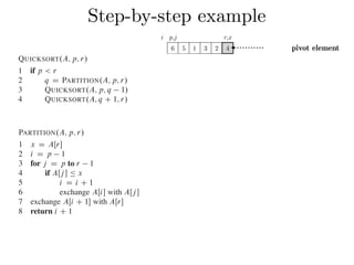
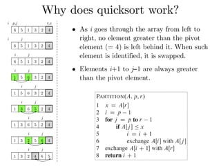
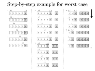
Figure 7.1 shows how PARTITION works on an 8-element array. PARTITION
always selects an element x D AŒr as a pivot element around which to partition the
subarray AŒp : : r. As the procedure runs, it partitions the array into four (possibly
empty) regions. At the start of each iteration of the for loop in lines 3–6, the regions
i j
6 5 1 3 2 4 x = 4, A[j = p+1] = 5 > x
i p,j r,x
6 5 1 3 2 4 pivot element](https://image.slidesharecdn.com/quicksort2019-190517113530/85/Quicksort-21-320.jpg)
![Step-by-step exampleCombine: Because the subarrays are already sorted, no work is needed to combine
them: the entire array AŒp : : r is now sorted.
The following procedure implements quicksort:
QUICKSORT.A; p; r/
1 if p < r
2 q D PARTITION.A; p; r/
3 QUICKSORT.A; p; q 1/
4 QUICKSORT.A; q C 1; r/
To sort an entire array A, the initial call is QUICKSORT.A; 1; A:length/.
Partitioning the array
The key to the algorithm is the PARTITION procedure, which rearranges the subar-
ray AŒp : : r in place.
PARTITION.A; p; r/
1 x D AŒr
2 i D p 1
3 for j D p to r 1
4 if AŒj Ä x
5 i D i C 1
6 exchange AŒi with AŒj
7 exchange AŒi C 1 with AŒr
8 return i C 1
QUICKSORT.A; p; r/
1 if p < r
2 q D PARTITION.A; p; r/
3 QUICKSORT.A; p; q 1/
4 QUICKSORT.A; q C 1; r/
To sort an entire array A, the initial call is QUICKSORT.A; 1; A:length/.
Partitioning the array
The key to the algorithm is the PARTITION procedure, which rearranges the subar-
ray AŒp : : r in place.
PARTITION.A; p; r/
1 x D AŒr
2 i D p 1
3 for j D p to r 1
4 if AŒj Ä x
5 i D i C 1
6 exchange AŒi with AŒj
7 exchange AŒi C 1 with AŒr
8 return i C 1
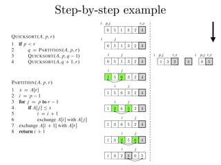
Figure 7.1 shows how PARTITION works on an 8-element array. PARTITION
always selects an element x D AŒr as a pivot element around which to partition the
subarray AŒp : : r. As the procedure runs, it partitions the array into four (possibly
empty) regions. At the start of each iteration of the for loop in lines 3–6, the regions
i j
6 5 1 3 2 4
i j
6 5 1 3 2 4
x = 4, A[j = p+1] = 5 > x
A[j = p+2] = 1 < x, i = i+1
i p,j r,x
6 5 1 3 2 4 pivot element](https://image.slidesharecdn.com/quicksort2019-190517113530/85/Quicksort-22-320.jpg)
![Step-by-step exampleCombine: Because the subarrays are already sorted, no work is needed to combine
them: the entire array AŒp : : r is now sorted.
The following procedure implements quicksort:
QUICKSORT.A; p; r/
1 if p < r
2 q D PARTITION.A; p; r/
3 QUICKSORT.A; p; q 1/
4 QUICKSORT.A; q C 1; r/
To sort an entire array A, the initial call is QUICKSORT.A; 1; A:length/.
Partitioning the array
The key to the algorithm is the PARTITION procedure, which rearranges the subar-
ray AŒp : : r in place.
PARTITION.A; p; r/
1 x D AŒr
2 i D p 1
3 for j D p to r 1
4 if AŒj Ä x
5 i D i C 1
6 exchange AŒi with AŒj
7 exchange AŒi C 1 with AŒr
8 return i C 1
QUICKSORT.A; p; r/
1 if p < r
2 q D PARTITION.A; p; r/
3 QUICKSORT.A; p; q 1/
4 QUICKSORT.A; q C 1; r/
To sort an entire array A, the initial call is QUICKSORT.A; 1; A:length/.
Partitioning the array
The key to the algorithm is the PARTITION procedure, which rearranges the subar-
ray AŒp : : r in place.
PARTITION.A; p; r/
1 x D AŒr
2 i D p 1
3 for j D p to r 1
4 if AŒj Ä x
5 i D i C 1
6 exchange AŒi with AŒj
7 exchange AŒi C 1 with AŒr
8 return i C 1
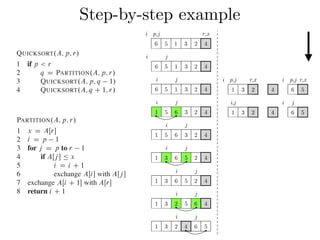
Figure 7.1 shows how PARTITION works on an 8-element array. PARTITION
always selects an element x D AŒr as a pivot element around which to partition the
subarray AŒp : : r. As the procedure runs, it partitions the array into four (possibly
empty) regions. At the start of each iteration of the for loop in lines 3–6, the regions
i j
6 5 1 3 2 4
i j
6 5 1 3 2 4
i j
1 5 6 3 2 4
x = 4, A[j = p+1] = 5 > x
A[j = p+2] = 1 < x, i = i+1
and A[i]↔A[j]
i p,j r,x
6 5 1 3 2 4 pivot element](https://image.slidesharecdn.com/quicksort2019-190517113530/85/Quicksort-23-320.jpg)
![Step-by-step exampleCombine: Because the subarrays are already sorted, no work is needed to combine
them: the entire array AŒp : : r is now sorted.
The following procedure implements quicksort:
QUICKSORT.A; p; r/
1 if p < r
2 q D PARTITION.A; p; r/
3 QUICKSORT.A; p; q 1/
4 QUICKSORT.A; q C 1; r/
To sort an entire array A, the initial call is QUICKSORT.A; 1; A:length/.
Partitioning the array
The key to the algorithm is the PARTITION procedure, which rearranges the subar-
ray AŒp : : r in place.
PARTITION.A; p; r/
1 x D AŒr
2 i D p 1
3 for j D p to r 1
4 if AŒj Ä x
5 i D i C 1
6 exchange AŒi with AŒj
7 exchange AŒi C 1 with AŒr
8 return i C 1
QUICKSORT.A; p; r/
1 if p < r
2 q D PARTITION.A; p; r/
3 QUICKSORT.A; p; q 1/
4 QUICKSORT.A; q C 1; r/
To sort an entire array A, the initial call is QUICKSORT.A; 1; A:length/.
Partitioning the array
The key to the algorithm is the PARTITION procedure, which rearranges the subar-
ray AŒp : : r in place.
PARTITION.A; p; r/
1 x D AŒr
2 i D p 1
3 for j D p to r 1
4 if AŒj Ä x
5 i D i C 1
6 exchange AŒi with AŒj
7 exchange AŒi C 1 with AŒr
8 return i C 1
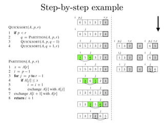
Figure 7.1 shows how PARTITION works on an 8-element array. PARTITION
always selects an element x D AŒr as a pivot element around which to partition the
subarray AŒp : : r. As the procedure runs, it partitions the array into four (possibly
empty) regions. At the start of each iteration of the for loop in lines 3–6, the regions
i j
6 5 1 3 2 4
i j
6 5 1 3 2 4
i j
1 5 6 3 2 4
i j
1 5 6 3 2 4
x = 4, A[j = p+1] = 5 > x
A[j = p+2] = 1 < x, i = i+1
and A[i]↔A[j]
A[j = p+3] = 3 < x, i = i+1
i p,j r,x
6 5 1 3 2 4 pivot element](https://image.slidesharecdn.com/quicksort2019-190517113530/85/Quicksort-24-320.jpg)
![Step-by-step exampleCombine: Because the subarrays are already sorted, no work is needed to combine
them: the entire array AŒp : : r is now sorted.
The following procedure implements quicksort:
QUICKSORT.A; p; r/
1 if p < r
2 q D PARTITION.A; p; r/
3 QUICKSORT.A; p; q 1/
4 QUICKSORT.A; q C 1; r/
To sort an entire array A, the initial call is QUICKSORT.A; 1; A:length/.
Partitioning the array
The key to the algorithm is the PARTITION procedure, which rearranges the subar-
ray AŒp : : r in place.
PARTITION.A; p; r/
1 x D AŒr
2 i D p 1
3 for j D p to r 1
4 if AŒj Ä x
5 i D i C 1
6 exchange AŒi with AŒj
7 exchange AŒi C 1 with AŒr
8 return i C 1
QUICKSORT.A; p; r/
1 if p < r
2 q D PARTITION.A; p; r/
3 QUICKSORT.A; p; q 1/
4 QUICKSORT.A; q C 1; r/
To sort an entire array A, the initial call is QUICKSORT.A; 1; A:length/.
Partitioning the array
The key to the algorithm is the PARTITION procedure, which rearranges the subar-
ray AŒp : : r in place.
PARTITION.A; p; r/
1 x D AŒr
2 i D p 1
3 for j D p to r 1
4 if AŒj Ä x
5 i D i C 1
6 exchange AŒi with AŒj
7 exchange AŒi C 1 with AŒr
8 return i C 1
Figure 7.1 shows how PARTITION works on an 8-element array. PARTITION
always selects an element x D AŒr as a pivot element around which to partition the
subarray AŒp : : r. As the procedure runs, it partitions the array into four (possibly
empty) regions. At the start of each iteration of the for loop in lines 3–6, the regions
i j
6 5 1 3 2 4
i j
6 5 1 3 2 4
i j
1 5 6 3 2 4
i j
1 5 6 3 2 4
i j
1 3 6 5 2 4
x = 4, A[j = p+1] = 5 > x
A[j = p+2] = 1 < x, i = i+1
and A[i]↔A[j]
A[j = p+3] = 3 < x, i = i+1
and A[i]↔A[j]
i p,j r,x
6 5 1 3 2 4 pivot element](https://image.slidesharecdn.com/quicksort2019-190517113530/85/Quicksort-25-320.jpg)
![Step-by-step exampleCombine: Because the subarrays are already sorted, no work is needed to combine
them: the entire array AŒp : : r is now sorted.
The following procedure implements quicksort:
QUICKSORT.A; p; r/
1 if p < r
2 q D PARTITION.A; p; r/
3 QUICKSORT.A; p; q 1/
4 QUICKSORT.A; q C 1; r/
To sort an entire array A, the initial call is QUICKSORT.A; 1; A:length/.
Partitioning the array
The key to the algorithm is the PARTITION procedure, which rearranges the subar-
ray AŒp : : r in place.
PARTITION.A; p; r/
1 x D AŒr
2 i D p 1
3 for j D p to r 1
4 if AŒj Ä x
5 i D i C 1
6 exchange AŒi with AŒj
7 exchange AŒi C 1 with AŒr
8 return i C 1
QUICKSORT.A; p; r/
1 if p < r
2 q D PARTITION.A; p; r/
3 QUICKSORT.A; p; q 1/
4 QUICKSORT.A; q C 1; r/
To sort an entire array A, the initial call is QUICKSORT.A; 1; A:length/.
Partitioning the array
The key to the algorithm is the PARTITION procedure, which rearranges the subar-
ray AŒp : : r in place.
PARTITION.A; p; r/
1 x D AŒr
2 i D p 1
3 for j D p to r 1
4 if AŒj Ä x
5 i D i C 1
6 exchange AŒi with AŒj
7 exchange AŒi C 1 with AŒr
8 return i C 1
Figure 7.1 shows how PARTITION works on an 8-element array. PARTITION
always selects an element x D AŒr as a pivot element around which to partition the
subarray AŒp : : r. As the procedure runs, it partitions the array into four (possibly
empty) regions. At the start of each iteration of the for loop in lines 3–6, the regions
i j
6 5 1 3 2 4
i j
6 5 1 3 2 4
i j
1 5 6 3 2 4
i j
1 5 6 3 2 4
i j
1 3 6 5 2 4
i j
1 3 6 5 2 4
x = 4, A[j = p+1] = 5 > x
A[j = p+2] = 1 < x, i = i+1
and A[i]↔A[j]
A[j = p+3] = 3 < x, i = i+1
and A[i]↔A[j]
i p,j r,x
6 5 1 3 2 4 pivot element](https://image.slidesharecdn.com/quicksort2019-190517113530/85/Quicksort-26-320.jpg)
![Step-by-step exampleCombine: Because the subarrays are already sorted, no work is needed to combine
them: the entire array AŒp : : r is now sorted.
The following procedure implements quicksort:
QUICKSORT.A; p; r/
1 if p < r
2 q D PARTITION.A; p; r/
3 QUICKSORT.A; p; q 1/
4 QUICKSORT.A; q C 1; r/
To sort an entire array A, the initial call is QUICKSORT.A; 1; A:length/.
Partitioning the array
The key to the algorithm is the PARTITION procedure, which rearranges the subar-
ray AŒp : : r in place.
PARTITION.A; p; r/
1 x D AŒr
2 i D p 1
3 for j D p to r 1
4 if AŒj Ä x
5 i D i C 1
6 exchange AŒi with AŒj
7 exchange AŒi C 1 with AŒr
8 return i C 1
QUICKSORT.A; p; r/
1 if p < r
2 q D PARTITION.A; p; r/
3 QUICKSORT.A; p; q 1/
4 QUICKSORT.A; q C 1; r/
To sort an entire array A, the initial call is QUICKSORT.A; 1; A:length/.
Partitioning the array
The key to the algorithm is the PARTITION procedure, which rearranges the subar-
ray AŒp : : r in place.
PARTITION.A; p; r/
1 x D AŒr
2 i D p 1
3 for j D p to r 1
4 if AŒj Ä x
5 i D i C 1
6 exchange AŒi with AŒj
7 exchange AŒi C 1 with AŒr
8 return i C 1
Figure 7.1 shows how PARTITION works on an 8-element array. PARTITION
always selects an element x D AŒr as a pivot element around which to partition the
subarray AŒp : : r. As the procedure runs, it partitions the array into four (possibly
empty) regions. At the start of each iteration of the for loop in lines 3–6, the regions
i j
6 5 1 3 2 4
i j
6 5 1 3 2 4
i j
1 5 6 3 2 4
i j
1 5 6 3 2 4
i j
1 3 6 5 2 4
i j
1 3 6 5 2 4
i j
1 3 2 5 6 4
x = 4, A[j = p+1] = 5 > x
A[j = p+2] = 1 < x, i = i+1
and A[i]↔A[j]
A[j = p+3] = 3 < x, i = i+1
and A[i]↔A[j]
i p,j r,x
6 5 1 3 2 4 pivot element](https://image.slidesharecdn.com/quicksort2019-190517113530/85/Quicksort-27-320.jpg)
![Step-by-step exampleCombine: Because the subarrays are already sorted, no work is needed to combine
them: the entire array AŒp : : r is now sorted.
The following procedure implements quicksort:
QUICKSORT.A; p; r/
1 if p < r
2 q D PARTITION.A; p; r/
3 QUICKSORT.A; p; q 1/
4 QUICKSORT.A; q C 1; r/
To sort an entire array A, the initial call is QUICKSORT.A; 1; A:length/.
Partitioning the array
The key to the algorithm is the PARTITION procedure, which rearranges the subar-
ray AŒp : : r in place.
PARTITION.A; p; r/
1 x D AŒr
2 i D p 1
3 for j D p to r 1
4 if AŒj Ä x
5 i D i C 1
6 exchange AŒi with AŒj
7 exchange AŒi C 1 with AŒr
8 return i C 1
QUICKSORT.A; p; r/
1 if p < r
2 q D PARTITION.A; p; r/
3 QUICKSORT.A; p; q 1/
4 QUICKSORT.A; q C 1; r/
To sort an entire array A, the initial call is QUICKSORT.A; 1; A:length/.
Partitioning the array
The key to the algorithm is the PARTITION procedure, which rearranges the subar-
ray AŒp : : r in place.
PARTITION.A; p; r/
1 x D AŒr
2 i D p 1
3 for j D p to r 1
4 if AŒj Ä x
5 i D i C 1
6 exchange AŒi with AŒj
7 exchange AŒi C 1 with AŒr
8 return i C 1
Figure 7.1 shows how PARTITION works on an 8-element array. PARTITION
always selects an element x D AŒr as a pivot element around which to partition the
subarray AŒp : : r. As the procedure runs, it partitions the array into four (possibly
empty) regions. At the start of each iteration of the for loop in lines 3–6, the regions
i j
6 5 1 3 2 4
i j
6 5 1 3 2 4
i j
1 5 6 3 2 4
i j
1 5 6 3 2 4
i j
1 3 6 5 2 4
i j
1 3 6 5 2 4
i j
1 3 2 5 6 4
i j
1 3 2 4 6 5
x = 4, A[j = p+1] = 5 > x
A[j = p+2] = 1 < x, i = i+1
and A[i]↔A[j]
A[j = p+3] = 3 < x, i = i+1
and A[i]↔A[j]
j = r−1, A[i+1]↔A[r]
i p,j r,x
6 5 1 3 2 4 pivot element](https://image.slidesharecdn.com/quicksort2019-190517113530/85/Quicksort-28-320.jpg)

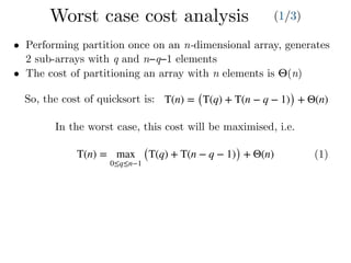
![• Instead of using the right-most element, A[r], as the pivot…
Randomised quicksort
element x D AŒr is equally likely to be any of the r p C 1 elements in the
subarray. Because we randomly choose the pivot element, we expect the split of
the input array to be reasonably well balanced on average.
The changes to PARTITION and QUICKSORT are small. In the new partition
procedure, we simply implement the swap before actually partitioning:
RANDOMIZED-PARTITION.A; p; r/
1 i D RANDOM.p; r/
2 exchange AŒr with AŒi
3 return PARTITION.A; p; r/
The new quicksort calls RANDOMIZED-PARTITION in place of PARTITION:
RANDOMIZED-QUICKSORT.A; p; r/
1 if p < r
2 q D RANDOMIZED-PARTITION.A; p; r/
3 RANDOMIZED-QUICKSORT.A; p; q 1/
4 RANDOMIZED-QUICKSORT.A; q C 1; r/
We analyze this algorithm in the next section.
subarray. Because we randomly choose the pivot element, we expect the split of
the input array to be reasonably well balanced on average.
The changes to PARTITION and QUICKSORT are small. In the new partition
procedure, we simply implement the swap before actually partitioning:
RANDOMIZED-PARTITION.A; p; r/
1 i D RANDOM.p; r/
2 exchange AŒr with AŒi
3 return PARTITION.A; p; r/
The new quicksort calls RANDOMIZED-PARTITION in place of PARTITION:
RANDOMIZED-QUICKSORT.A; p; r/
1 if p < r
2 q D RANDOMIZED-PARTITION.A; p; r/
3 RANDOMIZED-QUICKSORT.A; p; q 1/
4 RANDOMIZED-QUICKSORT.A; q C 1; r/
We analyze this algorithm in the next section.](https://image.slidesharecdn.com/quicksort2019-190517113530/85/Quicksort-79-320.jpg)
![• Instead of using the right-most element, A[r], as the pivot…
Randomised quicksort
element x D AŒr is equally likely to be any of the r p C 1 elements in the
subarray. Because we randomly choose the pivot element, we expect the split of
the input array to be reasonably well balanced on average.
The changes to PARTITION and QUICKSORT are small. In the new partition
procedure, we simply implement the swap before actually partitioning:
RANDOMIZED-PARTITION.A; p; r/
1 i D RANDOM.p; r/
2 exchange AŒr with AŒi
3 return PARTITION.A; p; r/
The new quicksort calls RANDOMIZED-PARTITION in place of PARTITION:
RANDOMIZED-QUICKSORT.A; p; r/
1 if p < r
2 q D RANDOMIZED-PARTITION.A; p; r/
3 RANDOMIZED-QUICKSORT.A; p; q 1/
4 RANDOMIZED-QUICKSORT.A; q C 1; r/
We analyze this algorithm in the next section.
subarray. Because we randomly choose the pivot element, we expect the split of
the input array to be reasonably well balanced on average.
The changes to PARTITION and QUICKSORT are small. In the new partition
procedure, we simply implement the swap before actually partitioning:
RANDOMIZED-PARTITION.A; p; r/
1 i D RANDOM.p; r/
2 exchange AŒr with AŒi
3 return PARTITION.A; p; r/
The new quicksort calls RANDOMIZED-PARTITION in place of PARTITION:
RANDOMIZED-QUICKSORT.A; p; r/
1 if p < r
2 q D RANDOMIZED-PARTITION.A; p; r/
3 RANDOMIZED-QUICKSORT.A; p; q 1/
4 RANDOMIZED-QUICKSORT.A; q C 1; r/
We analyze this algorithm in the next section.
• Why? By adding randomisation, obtaining the average expected
performance is more likely than obtaining the worst case
performance.](https://image.slidesharecdn.com/quicksort2019-190517113530/85/Quicksort-80-320.jpg)
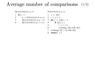
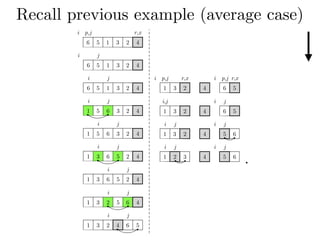
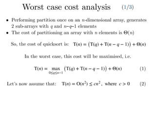
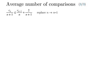
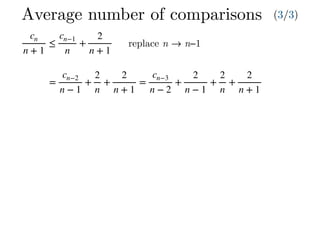
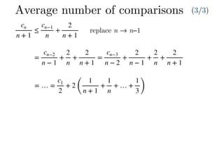
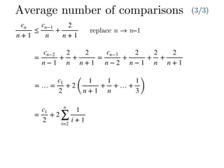
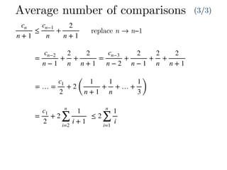
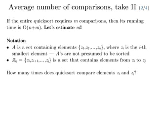
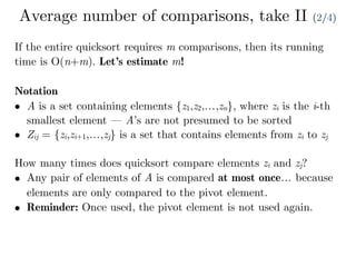
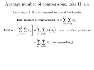
![Average number of comparisons (1/3)
cn = n +
1
n [(c0 + cn−1) + (c1 + cn−2) + … + (cn−1 + c0)]
Combine: Because the subarrays are already sorted, no work is needed to combine
them: the entire array AŒp : : r is now sorted.
The following procedure implements quicksort:
QUICKSORT.A; p; r/
1 if p < r
2 q D PARTITION.A; p; r/
3 QUICKSORT.A; p; q 1/
4 QUICKSORT.A; q C 1; r/
To sort an entire array A, the initial call is QUICKSORT.A; 1; A:length/.
Partitioning the array
The key to the algorithm is the PARTITION procedure, which rearranges the subar-
ray AŒp : : r in place.
PARTITION.A; p; r/
1 x D AŒr
2 i D p 1
3 for j D p to r 1
4 if AŒj Ä x
5 i D i C 1
6 exchange AŒi with AŒj
7 exchange AŒi C 1 with AŒr
8 return i C 1
Partitioning the array
The key to the algorithm is the PARTITION procedure, w
ray AŒp : : r in place.
PARTITION.A; p; r/
1 x D AŒr
2 i D p 1
3 for j D p to r 1
4 if AŒj Ä x
5 i D i C 1
6 exchange AŒi with AŒj
7 exchange AŒi C 1 with AŒr
8 return i C 1
Figure 7.1 shows how PARTITION works on an 8-e
always selects an element x D AŒr as a pivot element ar
subarray AŒp : : r. As the procedure runs, it partitions t
empty) regions. At the start of each iteration of the for lo
satisfy certain properties, shown in Figure 7.2. We stat
invariant:
At the beginning of each iteration of the loop of l
index k,
1. If p Ä k Ä i, then AŒk Ä x.
2. If i C 1 Ä k Ä j 1, then AŒk > x.
3. If k D r, then AŒk D x.](https://image.slidesharecdn.com/quicksort2019-190517113530/85/Quicksort-83-320.jpg)
![Average number of comparisons (1/3)
cn = n +
1
n [(c0 + cn−1) + (c1 + cn−2) + … + (cn−1 + c0)]
Combine: Because the subarrays are already sorted, no work is needed to combine
them: the entire array AŒp : : r is now sorted.
The following procedure implements quicksort:
QUICKSORT.A; p; r/
1 if p < r
2 q D PARTITION.A; p; r/
3 QUICKSORT.A; p; q 1/
4 QUICKSORT.A; q C 1; r/
To sort an entire array A, the initial call is QUICKSORT.A; 1; A:length/.
Partitioning the array
The key to the algorithm is the PARTITION procedure, which rearranges the subar-
ray AŒp : : r in place.
PARTITION.A; p; r/
1 x D AŒr
2 i D p 1
3 for j D p to r 1
4 if AŒj Ä x
5 i D i C 1
6 exchange AŒi with AŒj
7 exchange AŒi C 1 with AŒr
8 return i C 1
Partitioning the array
The key to the algorithm is the PARTITION procedure, w
ray AŒp : : r in place.
PARTITION.A; p; r/
1 x D AŒr
2 i D p 1
3 for j D p to r 1
4 if AŒj Ä x
5 i D i C 1
6 exchange AŒi with AŒj
7 exchange AŒi C 1 with AŒr
8 return i C 1
Figure 7.1 shows how PARTITION works on an 8-e
always selects an element x D AŒr as a pivot element ar
subarray AŒp : : r. As the procedure runs, it partitions t
empty) regions. At the start of each iteration of the for lo
satisfy certain properties, shown in Figure 7.2. We stat
invariant:
At the beginning of each iteration of the loop of l
index k,
1. If p Ä k Ä i, then AŒk Ä x.
2. If i C 1 Ä k Ä j 1, then AŒk > x.
3. If k D r, then AŒk D x.
total number of
comparisons](https://image.slidesharecdn.com/quicksort2019-190517113530/85/Quicksort-84-320.jpg)
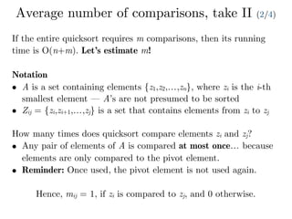
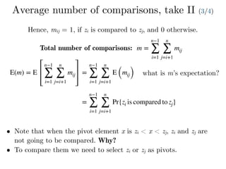
![Average number of comparisons (1/3)
cn = n +
1
n [(c0 + cn−1) + (c1 + cn−2) + … + (cn−1 + c0)]
Combine: Because the subarrays are already sorted, no work is needed to combine
them: the entire array AŒp : : r is now sorted.
The following procedure implements quicksort:
QUICKSORT.A; p; r/
1 if p < r
2 q D PARTITION.A; p; r/
3 QUICKSORT.A; p; q 1/
4 QUICKSORT.A; q C 1; r/
To sort an entire array A, the initial call is QUICKSORT.A; 1; A:length/.
Partitioning the array
The key to the algorithm is the PARTITION procedure, which rearranges the subar-
ray AŒp : : r in place.
PARTITION.A; p; r/
1 x D AŒr
2 i D p 1
3 for j D p to r 1
4 if AŒj Ä x
5 i D i C 1
6 exchange AŒi with AŒj
7 exchange AŒi C 1 with AŒr
8 return i C 1
Partitioning the array
The key to the algorithm is the PARTITION procedure, w
ray AŒp : : r in place.
PARTITION.A; p; r/
1 x D AŒr
2 i D p 1
3 for j D p to r 1
4 if AŒj Ä x
5 i D i C 1
6 exchange AŒi with AŒj
7 exchange AŒi C 1 with AŒr
8 return i C 1
Figure 7.1 shows how PARTITION works on an 8-e
always selects an element x D AŒr as a pivot element ar
subarray AŒp : : r. As the procedure runs, it partitions t
empty) regions. At the start of each iteration of the for lo
satisfy certain properties, shown in Figure 7.2. We stat
invariant:
At the beginning of each iteration of the loop of l
index k,
1. If p Ä k Ä i, then AŒk Ä x.
2. If i C 1 Ä k Ä j 1, then AŒk > x.
3. If k D r, then AŒk D x.
total number of
comparisons
probability of a
split — n pivot
choices](https://image.slidesharecdn.com/quicksort2019-190517113530/85/Quicksort-85-320.jpg)
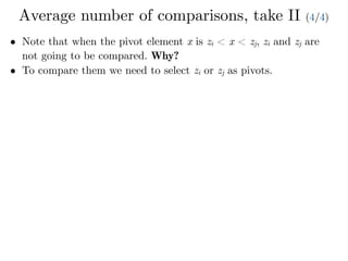
![Average number of comparisons (1/3)
cn = n +
1
n [(c0 + cn−1) + (c1 + cn−2) + … + (cn−1 + c0)]
Combine: Because the subarrays are already sorted, no work is needed to combine
them: the entire array AŒp : : r is now sorted.
The following procedure implements quicksort:
QUICKSORT.A; p; r/
1 if p < r
2 q D PARTITION.A; p; r/
3 QUICKSORT.A; p; q 1/
4 QUICKSORT.A; q C 1; r/
To sort an entire array A, the initial call is QUICKSORT.A; 1; A:length/.
Partitioning the array
The key to the algorithm is the PARTITION procedure, which rearranges the subar-
ray AŒp : : r in place.
PARTITION.A; p; r/
1 x D AŒr
2 i D p 1
3 for j D p to r 1
4 if AŒj Ä x
5 i D i C 1
6 exchange AŒi with AŒj
7 exchange AŒi C 1 with AŒr
8 return i C 1
Partitioning the array
The key to the algorithm is the PARTITION procedure, w
ray AŒp : : r in place.
PARTITION.A; p; r/
1 x D AŒr
2 i D p 1
3 for j D p to r 1
4 if AŒj Ä x
5 i D i C 1
6 exchange AŒi with AŒj
7 exchange AŒi C 1 with AŒr
8 return i C 1
Figure 7.1 shows how PARTITION works on an 8-e
always selects an element x D AŒr as a pivot element ar
subarray AŒp : : r. As the procedure runs, it partitions t
empty) regions. At the start of each iteration of the for lo
satisfy certain properties, shown in Figure 7.2. We stat
invariant:
At the beginning of each iteration of the loop of l
index k,
1. If p Ä k Ä i, then AŒk Ä x.
2. If i C 1 Ä k Ä j 1, then AŒk > x.
3. If k D r, then AŒk D x.
total number of
comparisons
probability of a
split — n pivot
choices
sub-array sizes](https://image.slidesharecdn.com/quicksort2019-190517113530/85/Quicksort-86-320.jpg)
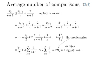
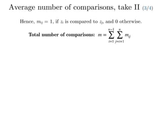
![cn = n +
1
n [(c0 + cn−1) + (c1 + cn−2) + … + (cn−1 + c0)]
= n +
2
n
(c0 + c1 + … + cn−1) ⟹
Average number of comparisons (2/3)](https://image.slidesharecdn.com/quicksort2019-190517113530/85/Quicksort-87-320.jpg)
![cn = n +
1
n [(c0 + cn−1) + (c1 + cn−2) + … + (cn−1 + c0)]
= n +
2
n
(c0 + c1 + … + cn−1) ⟹
ncn = n2
+ 2 (c0 + c1 + … + cn−1)
Average number of comparisons (2/3)](https://image.slidesharecdn.com/quicksort2019-190517113530/85/Quicksort-88-320.jpg)
![cn = n +
1
n [(c0 + cn−1) + (c1 + cn−2) + … + (cn−1 + c0)]
= n +
2
n
(c0 + c1 + … + cn−1) ⟹
ncn = n2
+ 2 (c0 + c1 + … + cn−1)
(n − 1)cn−1 = (n − 1)2
+ 2 (c0 + c1 + … + cn−2)
Average number of comparisons (2/3)
Replace n → n−1](https://image.slidesharecdn.com/quicksort2019-190517113530/85/Quicksort-89-320.jpg)
![cn = n +
1
n [(c0 + cn−1) + (c1 + cn−2) + … + (cn−1 + c0)]
= n +
2
n
(c0 + c1 + … + cn−1) ⟹
ncn = n2
+ 2 (c0 + c1 + … + cn−1)
(n − 1)cn−1 = (n − 1)2
+ 2 (c0 + c1 + … + cn−2)
Average number of comparisons (2/3)
subtract](https://image.slidesharecdn.com/quicksort2019-190517113530/85/Quicksort-90-320.jpg)
![cn = n +
1
n [(c0 + cn−1) + (c1 + cn−2) + … + (cn−1 + c0)]
= n +
2
n
(c0 + c1 + … + cn−1) ⟹
ncn = n2
+ 2 (c0 + c1 + … + cn−1)
(n − 1)cn−1 = (n − 1)2
+ 2 (c0 + c1 + … + cn−2)
ncn − (n − 1)cn−1 = 2(n − 1) + 2cn−1 ⟹
Average number of comparisons (2/3)
subtract](https://image.slidesharecdn.com/quicksort2019-190517113530/85/Quicksort-91-320.jpg)
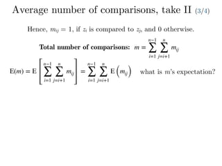
![cn = n +
1
n [(c0 + cn−1) + (c1 + cn−2) + … + (cn−1 + c0)]
= n +
2
n
(c0 + c1 + … + cn−1) ⟹
ncn = n2
+ 2 (c0 + c1 + … + cn−1)
(n − 1)cn−1 = (n − 1)2
+ 2 (c0 + c1 + … + cn−2)
ncn − (n − 1)cn−1 = 2(n − 1) + 2cn−1 ⟹
Average number of comparisons (2/3)
subtract
cn =
2n − 1
n
+
(n + 1)cn−1
n
⟹](https://image.slidesharecdn.com/quicksort2019-190517113530/85/Quicksort-92-320.jpg)
![cn = n +
1
n [(c0 + cn−1) + (c1 + cn−2) + … + (cn−1 + c0)]
= n +
2
n
(c0 + c1 + … + cn−1) ⟹
ncn = n2
+ 2 (c0 + c1 + … + cn−1)
(n − 1)cn−1 = (n − 1)2
+ 2 (c0 + c1 + … + cn−2)
ncn − (n − 1)cn−1 = 2(n − 1) + 2cn−1 ⟹
Average number of comparisons (2/3)
subtract
cn =
2n − 1
n
+
(n + 1)cn−1
n
⟹ divide by n + 1](https://image.slidesharecdn.com/quicksort2019-190517113530/85/Quicksort-93-320.jpg)
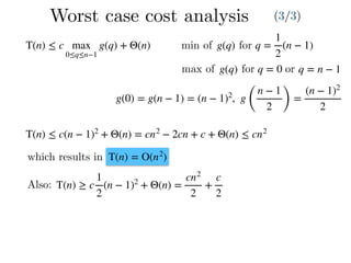
![cn = n +
1
n [(c0 + cn−1) + (c1 + cn−2) + … + (cn−1 + c0)]
= n +
2
n
(c0 + c1 + … + cn−1) ⟹
ncn = n2
+ 2 (c0 + c1 + … + cn−1)
(n − 1)cn−1 = (n − 1)2
+ 2 (c0 + c1 + … + cn−2)
ncn − (n − 1)cn−1 = 2(n − 1) + 2cn−1 ⟹
cn
n + 1
=
2
n + 1
−
1
n(n + 1)
+
cn−1
n
Average number of comparisons (2/3)
subtract
cn =
2n − 1
n
+
(n + 1)cn−1
n
⟹ divide by n + 1](https://image.slidesharecdn.com/quicksort2019-190517113530/85/Quicksort-94-320.jpg)
![cn = n +
1
n [(c0 + cn−1) + (c1 + cn−2) + … + (cn−1 + c0)]
= n +
2
n
(c0 + c1 + … + cn−1) ⟹
ncn = n2
+ 2 (c0 + c1 + … + cn−1)
(n − 1)cn−1 = (n − 1)2
+ 2 (c0 + c1 + … + cn−2)
ncn − (n − 1)cn−1 = 2(n − 1) + 2cn−1 ⟹
cn
n + 1
=
2
n + 1
−
1
n(n + 1)
+
cn−1
n
Average number of comparisons (2/3)
subtract
cn =
2n − 1
n
+
(n + 1)cn−1
n
⟹ divide by n + 1
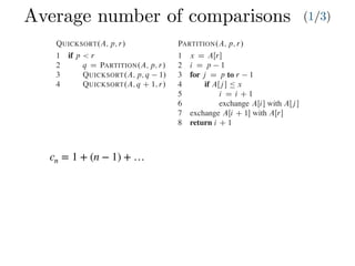
≤
2
n + 1
+
cn−1
n](https://image.slidesharecdn.com/quicksort2019-190517113530/85/Quicksort-95-320.jpg)

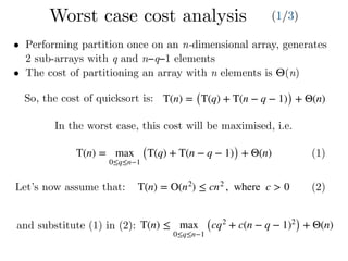
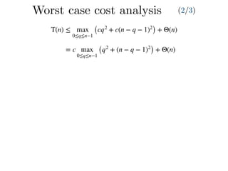
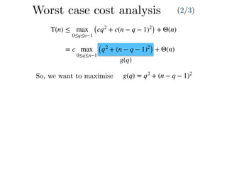
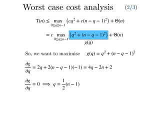
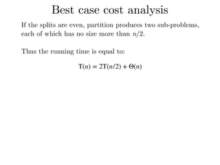
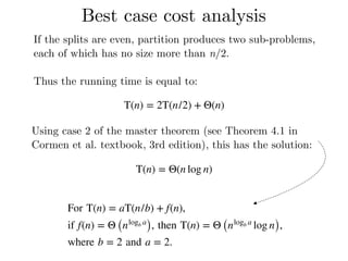
The document covers the Quicksort algorithm, a divide-and-conquer sorting method that efficiently sorts an array by partitioning elements around a pivot. Originating from Tony Hoare's work in 1959, it has an average time complexity of O(n log n), requiring minimal memory as it operates in place. It details the steps of partitioning and recursive sorting of sub-arrays, culminating in a sorted array.


![ppt daaa[1].pptxdaaaaaaaaaaaaaaaaaaaaaaaaaaaaaaaaa](https://cdn.slidesharecdn.com/ss_thumbnails/pptdaaa1-251211161628-1cb28a51-thumbnail.jpg?width=640&height=640&fit=bounds)