Introduction to Algorithms
Quicksort
CSE 680
Prof. Roger Crawfis
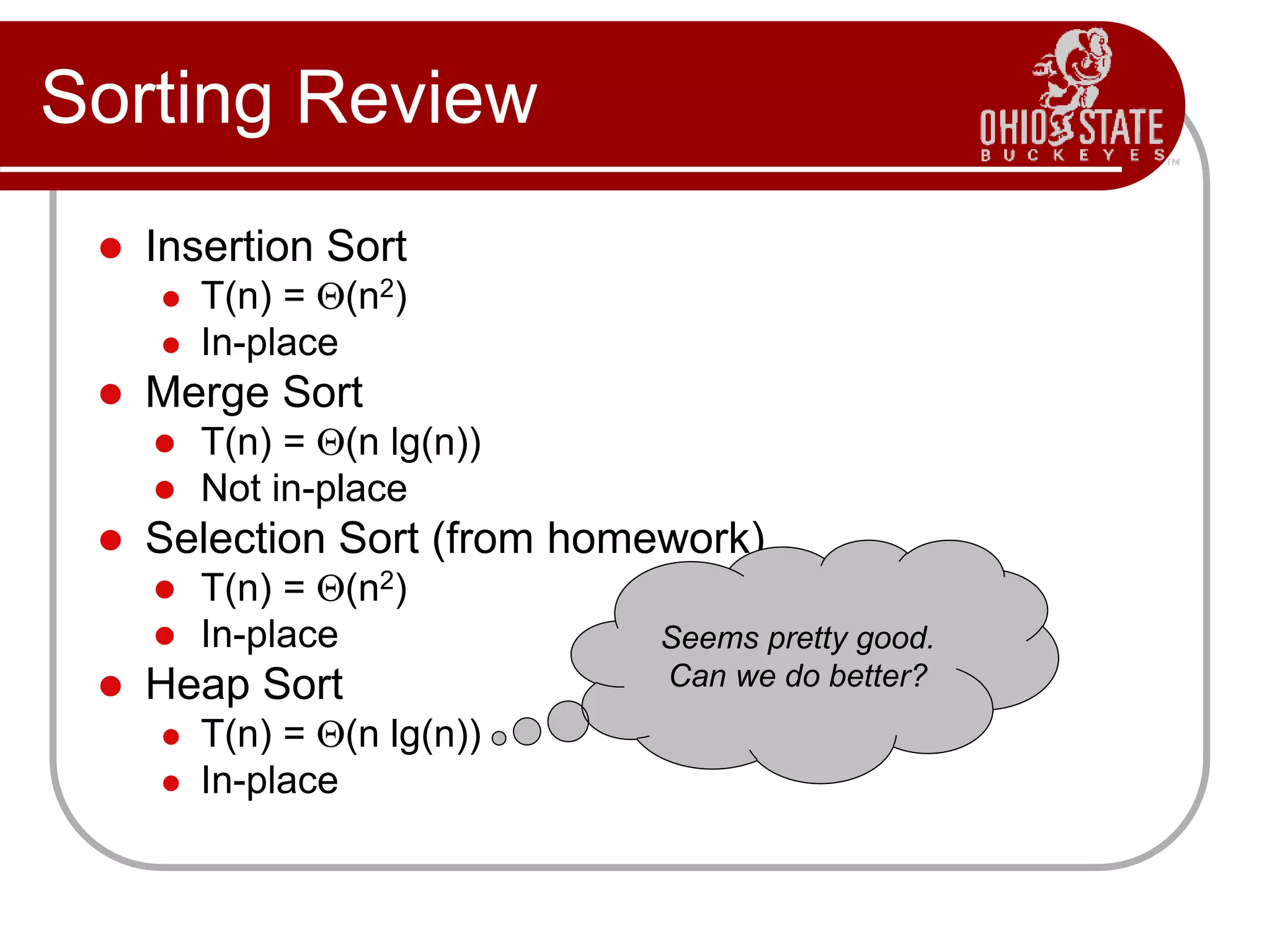
Sorting Review
 Insertion Sort
 T(n) = Q(n2)
 In-place
 Merge Sort
 T(n) = Q(n lg(n))
 Not in-place
 Selection Sort (from homework)
 T(n) = Q(n2)
 In-place
 Heap Sort
 T(n) = Q(n lg(n))
 In-place
Seems pretty good.
Can we do better?
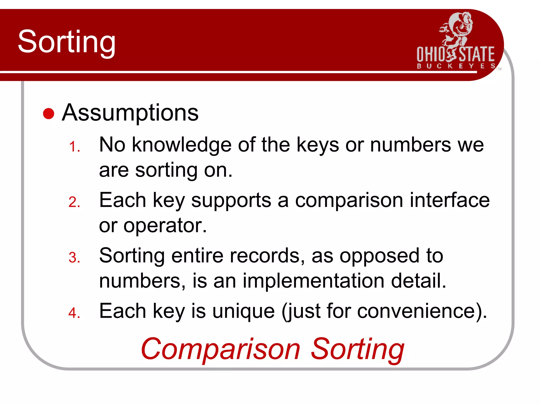
Sorting
 Assumptions
1. No knowledge of the keys or numbers we
are sorting on.
2. Each key supports a comparison interface
or operator.
3. Sorting entire records, as opposed to
numbers, is an implementation detail.
4. Each key is unique (just for convenience).
Comparison Sorting
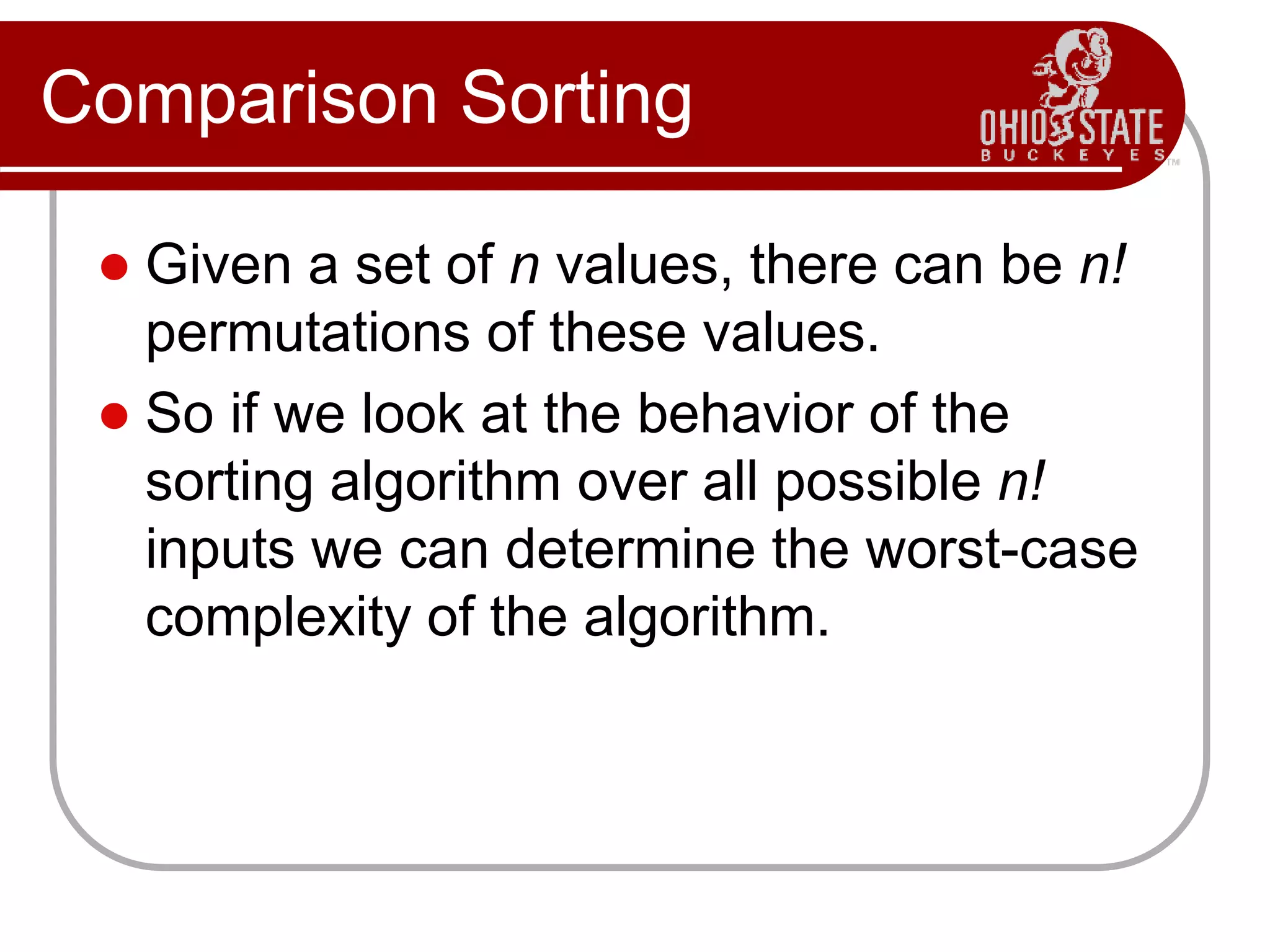
Comparison Sorting
 Given a set of n values, there can be n!
permutations of these values.
 So if we look at the behavior of the
sorting algorithm over all possible n!
inputs we can determine the worst-case
complexity of the algorithm.
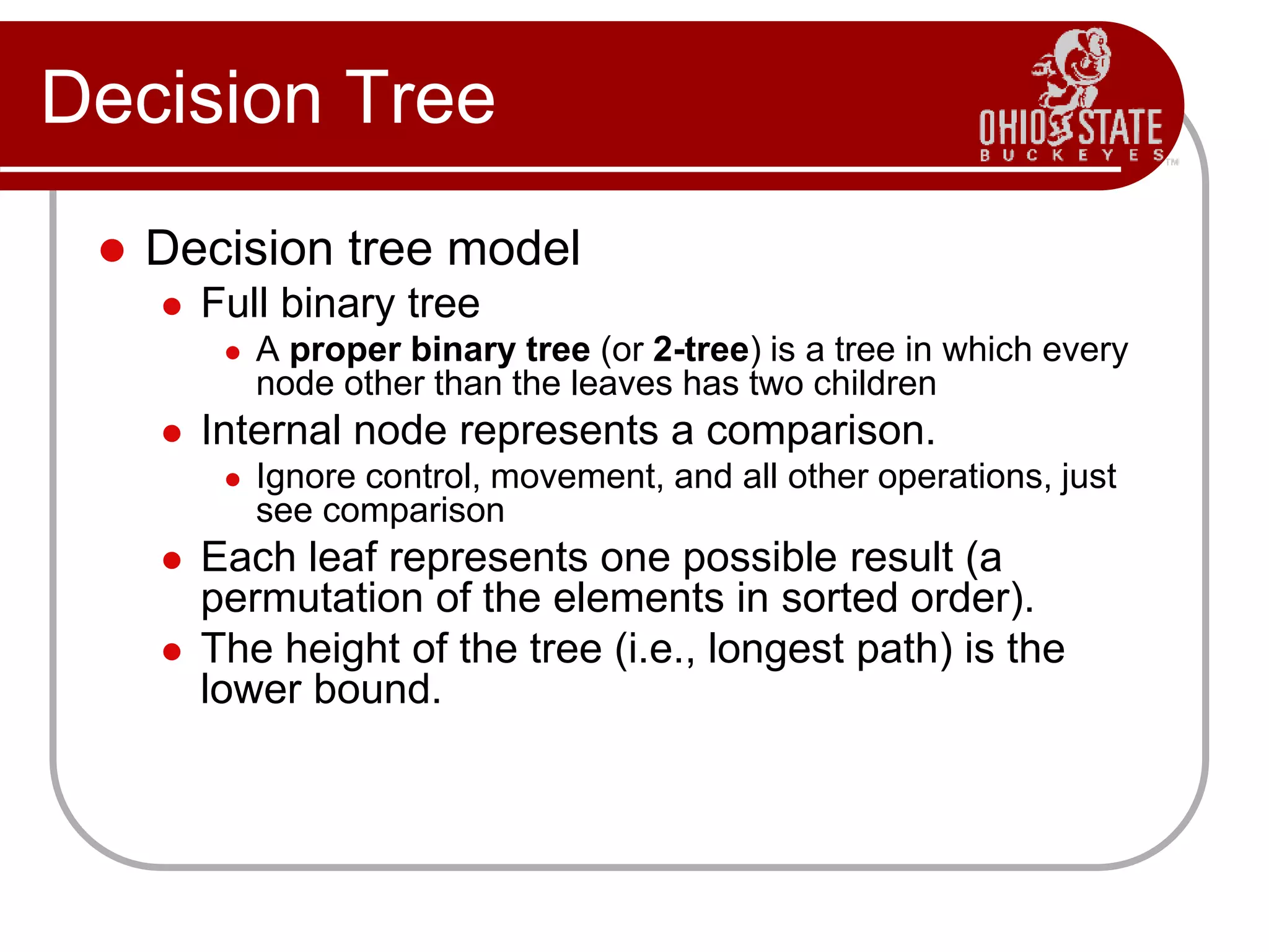
Decision Tree
 Decision tree model
 Full binary tree
 A proper binary tree (or 2-tree) is a tree in which every
node other than the leaves has two children
 Internal node represents a comparison.
 Ignore control, movement, and all other operations, just
see comparison
 Each leaf represents one possible result (a
permutation of the elements in sorted order).
 The height of the tree (i.e., longest path) is the
lower bound.
Decision Tree Model
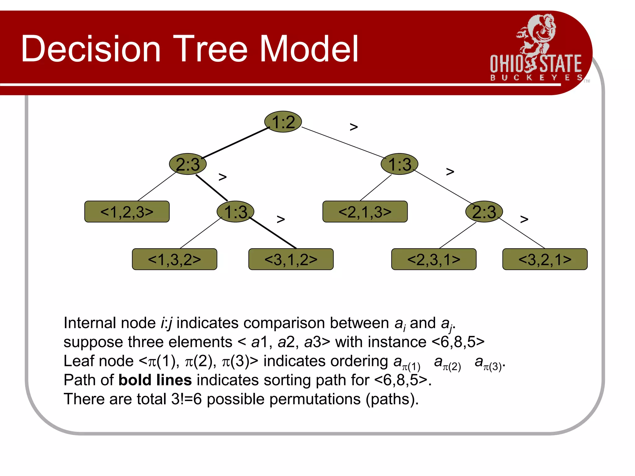
2:3
1:2
2:3
1:3
1:3
<1,2,3>
<1,3,2> <3,1,2>
<2,1,3>
<2,3,1> <3,2,1>

 

>
>
>
>
>
Internal node i:j indicates comparison between ai and aj.
suppose three elements < a1, a2, a3> with instance <6,8,5>
Leaf node <(1), (2), (3)> indicates ordering a(1) a(2) a(3).
Path of bold lines indicates sorting path for <6,8,5>.
There are total 3!=6 possible permutations (paths).

Decision Tree Model
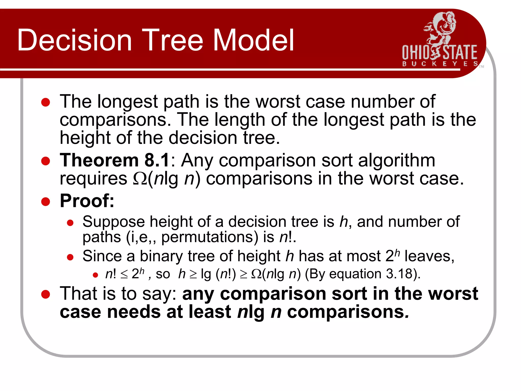
 The longest path is the worst case number of
comparisons. The length of the longest path is the
height of the decision tree.
 Theorem 8.1: Any comparison sort algorithm
requires (nlg n) comparisons in the worst case.
 Proof:
 Suppose height of a decision tree is h, and number of
paths (i,e,, permutations) is n!.
 Since a binary tree of height h has at most 2h leaves,
 n!  2h , so h  lg (n!)  (nlg n) (By equation 3.18).
 That is to say: any comparison sort in the worst
case needs at least nlg n comparisons.
QuickSort Design
 Follows the divide-and-conquer paradigm.
 Divide: Partition (separate) the array A[p..r] into two
(possibly empty) subarrays A[p..q–1] and A[q+1..r].
 Each element in A[p..q–1] < A[q].
 A[q] < each element in A[q+1..r].
 Index q is computed as part of the partitioning procedure.
 Conquer: Sort the two subarrays by recursive calls to
quicksort.
 Combine: The subarrays are sorted in place – no
work is needed to combine them.
 How do the divide and combine steps of quicksort
compare with those of merge sort?
Pseudocode
Quicksort(A, p, r)
if p < r then
q := Partition(A, p, r);
Quicksort(A, p, q – 1);
Quicksort(A, q + 1, r)
Partition(A, p, r)
x, i := A[r], p – 1;
for j := p to r – 1 do
if A[j]  x then
i := i + 1;
A[i]  A[j]
A[i + 1]  A[r];
return i + 1
5
A[p..r]
A[p..q – 1] A[q+1..r]
 5  5
Partition
5
Example
p r
initially: 2 5 8 3 9 4 1 7 10 6 note: pivot (x) = 6
i j
next iteration: 2 5 8 3 9 4 1 7 10 6
i j
next iteration: 2 5 8 3 9 4 1 7 10 6
i j
next iteration: 2 5 8 3 9 4 1 7 10 6
i j
next iteration: 2 5 3 8 9 4 1 7 10 6
i j
Partition(A, p, r)
x, i := A[r], p – 1;
for j := p to r – 1 do
if A[j]  x then
i := i + 1;
A[i]  A[j]
A[i + 1]  A[r];
return i + 1
Example (Continued)
next iteration: 2 5 3 8 9 4 1 7 10 6
i j
next iteration: 2 5 3 8 9 4 1 7 10 6
i j
next iteration: 2 5 3 4 9 8 1 7 10 6
i j
next iteration: 2 5 3 4 1 8 9 7 10 6
i j
next iteration: 2 5 3 4 1 8 9 7 10 6
i j
next iteration: 2 5 3 4 1 8 9 7 10 6
i j
after final swap: 2 5 3 4 1 6 9 7 10 8
i j
Partition(A, p, r)
x, i := A[r], p – 1;
for j := p to r – 1 do
if A[j]  x then
i := i + 1;
A[i]  A[j]
A[i + 1]  A[r];
return i + 1
Partitioning
 Select the last element A[r] in the subarray
A[p..r] as the pivot – the element around which
to partition.
 As the procedure executes, the array is
partitioned into four (possibly empty) regions.
1. A[p..i ] — All entries in this region are < pivot.
2. A[i+1..j – 1] — All entries in this region are > pivot.
3. A[r] = pivot.
4. A[j..r – 1] — Not known how they compare to pivot.
 The above hold before each iteration of the for
loop, and constitute a loop invariant. (4 is not part
of the loopi.)
Correctness of Partition
 Use loop invariant.
 Initialization:
 Before first iteration
 A[p..i] and A[i+1..j – 1] are empty – Conds. 1 and 2 are satisfied
(trivially).
 r is the index of the pivot
 Cond. 3 is satisfied.
 Maintenance:
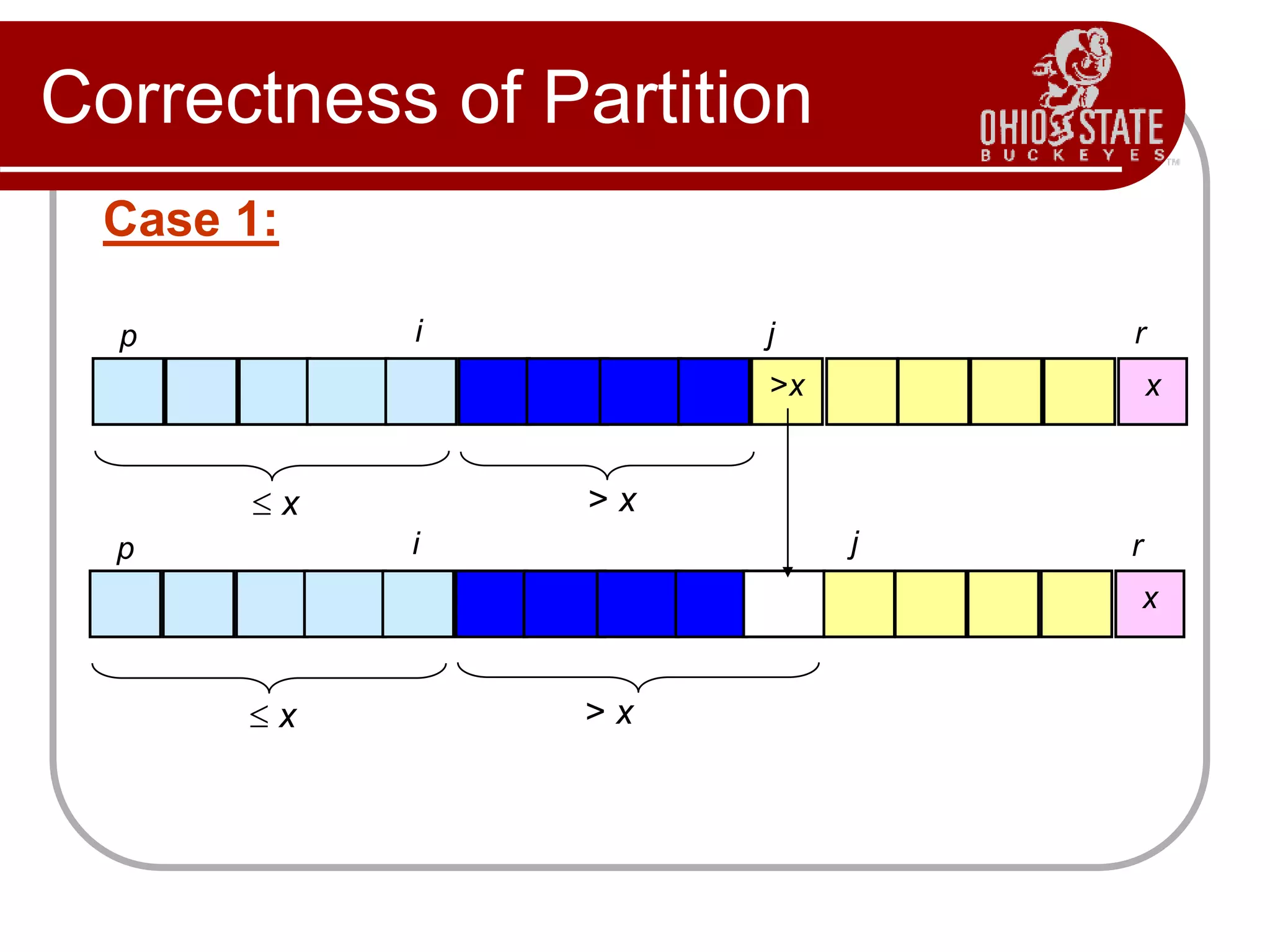
 Case 1: A[j] > x
 Increment j only.
 Loop Invariant is maintained.
Partition(A, p, r)
x, i := A[r], p – 1;
for j := p to r – 1 do
if A[j]  x then
i := i + 1;
A[i]  A[j]
A[i + 1]  A[r];
return i + 1
Correctness of Partition
>x x
p i j r
 x > x
x
p i j r
 x > x
Case 1:
Correctness of Partition
 Case 2: A[j]  x
 Increment i
 Swap A[i] and A[j]
 Condition 1 is
maintained.
 Increment j
 Condition 2 is
maintained.
 A[r] is unaltered.
 Condition 3 is
maintained.
 x x
p i j r
 x > x
 x > x
x
p i j r
Correctness of Partition
 Termination:
 When the loop terminates, j = r, so all elements
in A are partitioned into one of the three cases:
 A[p..i]  pivot
 A[i+1..j – 1] > pivot
 A[r] = pivot
 The last two lines swap A[i+1] and A[r].
 Pivot moves from the end of the array to
between the two subarrays.
 Thus, procedure partition correctly performs
the divide step.
Complexity of Partition
 PartitionTime(n) is given by the number
of iterations in the for loop.
 Q(n) : n = r – p + 1.
Partition(A, p, r)
x, i := A[r], p – 1;
for j := p to r – 1 do
if A[j]  x then
i := i + 1;
A[i]  A[j]
A[i + 1]  A[r];
return i + 1
Quicksort Overview
 To sort a[left...right]:
1. if left < right:
1.1. Partition a[left...right] such that:
all a[left...p-1] are less than a[p], and
all a[p+1...right] are >= a[p]
1.2. Quicksort a[left...p-1]
1.3. Quicksort a[p+1...right]
2. Terminate
Partitioning in Quicksort
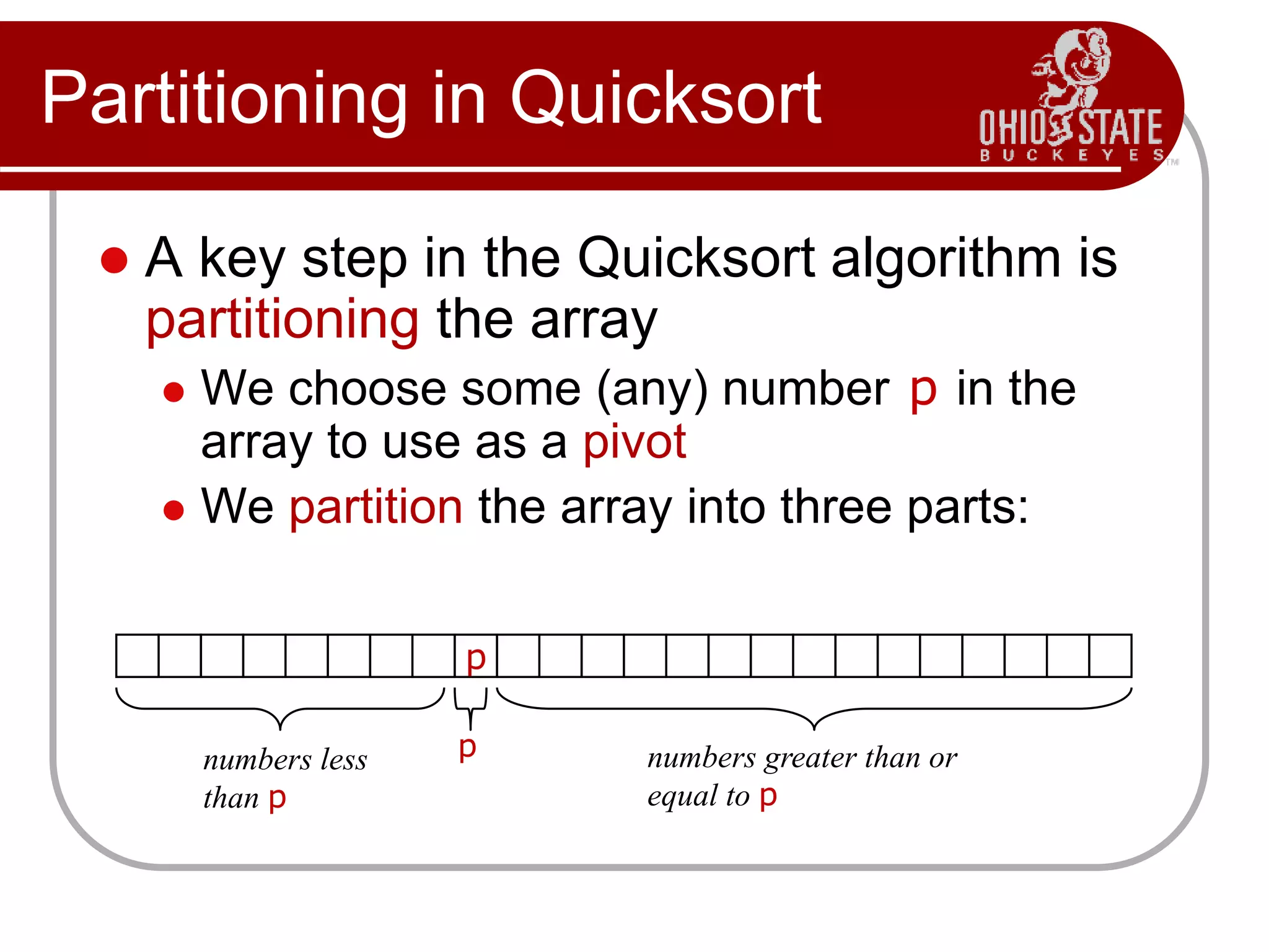
 A key step in the Quicksort algorithm is
partitioning the array
 We choose some (any) number p in the
array to use as a pivot
 We partition the array into three parts:
p
numbers less
than p
numbers greater than or
equal to p
p
Alternative Partitioning
 Choose an array value (say, the first) to use
as the pivot
 Starting from the left end, find the first
element that is greater than or equal to the
pivot
 Searching backward from the right end, find
the first element that is less than the pivot
 Interchange (swap) these two elements
 Repeat, searching from where we left off,
until done
Alternative Partitioning
 To partition a[left...right]:
1. Set pivot = a[left], l = left + 1, r = right;
2. while l < r, do
2.1. while l < right & a[l] < pivot , set l = l + 1
2.2. while r > left & a[r] >= pivot , set r = r - 1
2.3. if l < r, swap a[l] and a[r]
3. Set a[left] = a[r], a[r] = pivot
4. Terminate
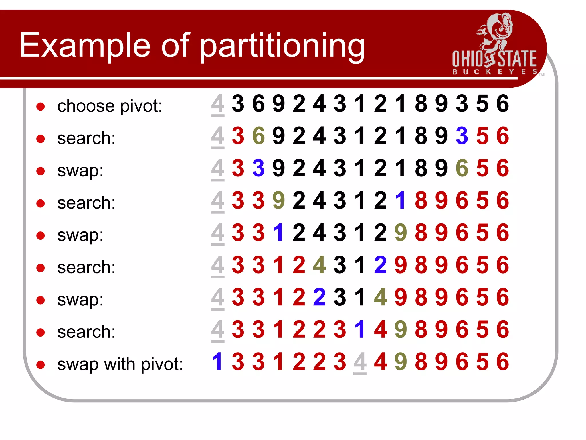
Example of partitioning
 choose pivot: 4 3 6 9 2 4 3 1 2 1 8 9 3 5 6
 search: 4 3 6 9 2 4 3 1 2 1 8 9 3 5 6
 swap: 4 3 3 9 2 4 3 1 2 1 8 9 6 5 6
 search: 4 3 3 9 2 4 3 1 2 1 8 9 6 5 6
 swap: 4 3 3 1 2 4 3 1 2 9 8 9 6 5 6
 search: 4 3 3 1 2 4 3 1 2 9 8 9 6 5 6
 swap: 4 3 3 1 2 2 3 1 4 9 8 9 6 5 6
 search: 4 3 3 1 2 2 3 1 4 9 8 9 6 5 6
 swap with pivot: 1 3 3 1 2 2 3 4 4 9 8 9 6 5 6
Partition Implementation (Java)
static int Partition(int[] a, int left, int right) {
int p = a[left], l = left + 1, r = right;
while (l < r) {
while (l < right && a[l] < p) l++;
while (r > left && a[r] >= p) r--;
if (l < r) {
int temp = a[l]; a[l] = a[r]; a[r] = temp;
}
}
a[left] = a[r];
a[r] = p;
return r;
}
Quicksort Implementation (Java)
static void Quicksort(int[] array, int left, int right)
{
if (left < right) {
int p = Partition(array, left, right);
Quicksort(array, left, p - 1);
Quicksort(array, p + 1, right);
}
}
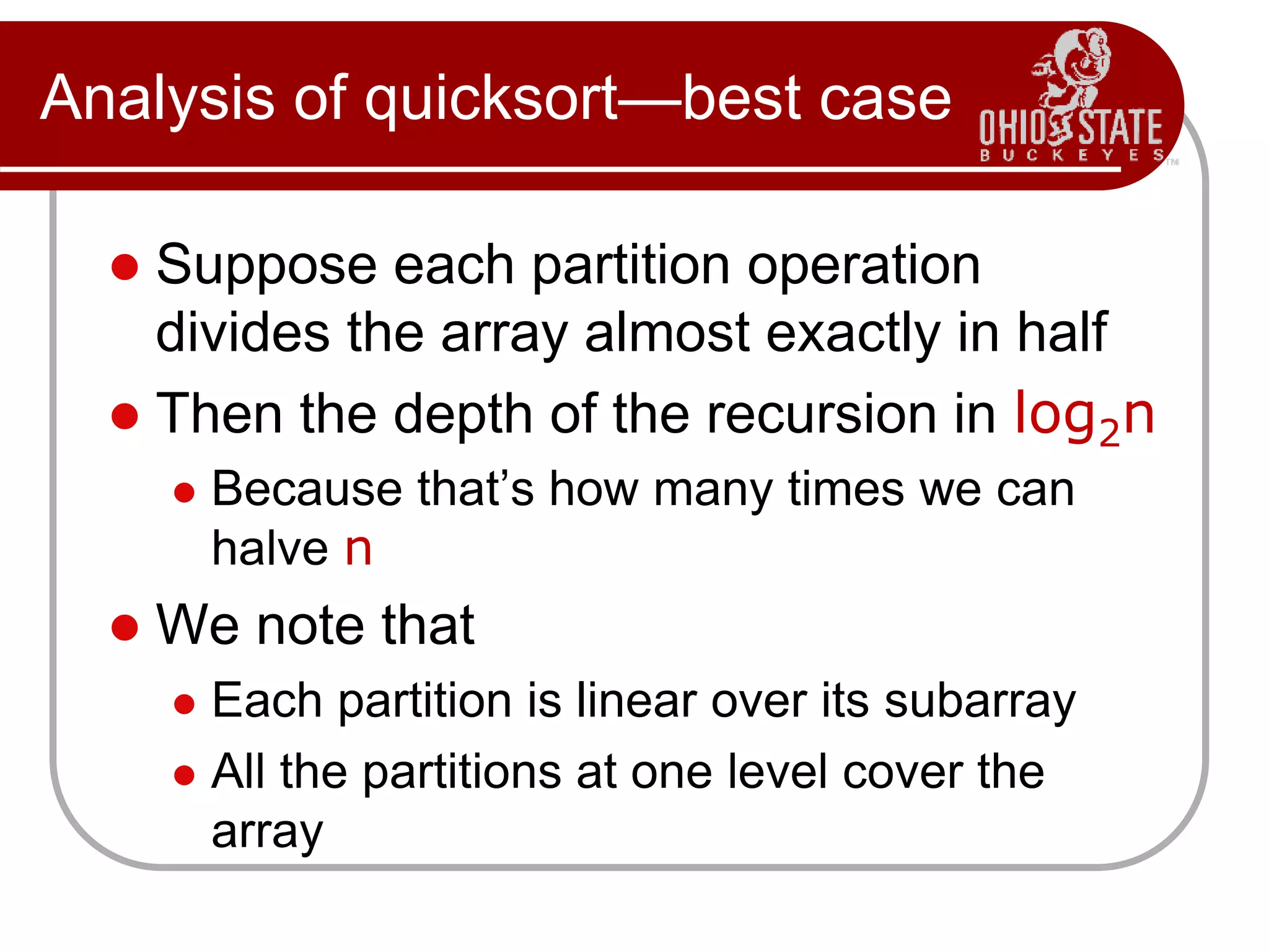
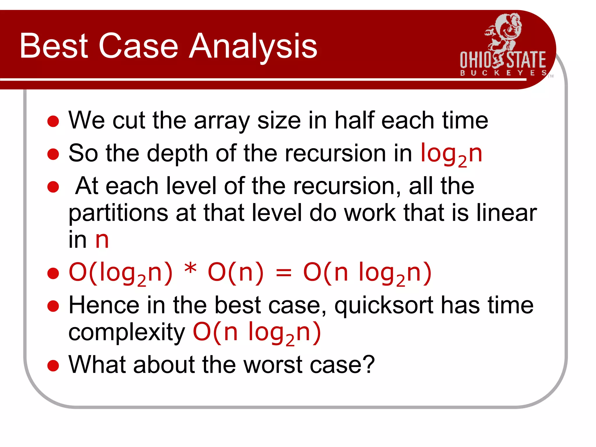
Analysis of quicksort—best case
 Suppose each partition operation
divides the array almost exactly in half
 Then the depth of the recursion in log2n
 Because that’s how many times we can
halve n
 We note that
 Each partition is linear over its subarray
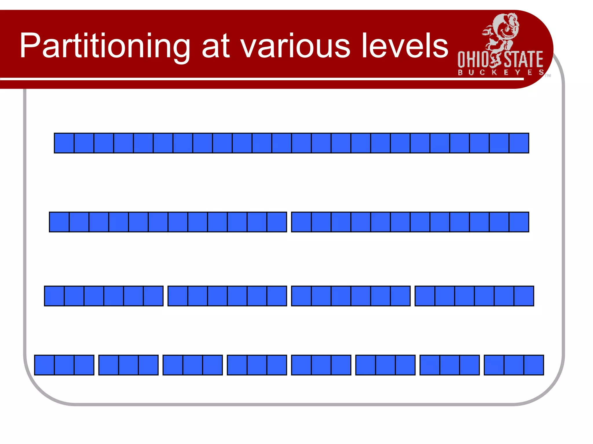
 All the partitions at one level cover the
array
Partitioning at various levels
Best Case Analysis
 We cut the array size in half each time
 So the depth of the recursion in log2n
 At each level of the recursion, all the
partitions at that level do work that is linear
in n
 O(log2n) * O(n) = O(n log2n)
 Hence in the best case, quicksort has time
complexity O(n log2n)
 What about the worst case?
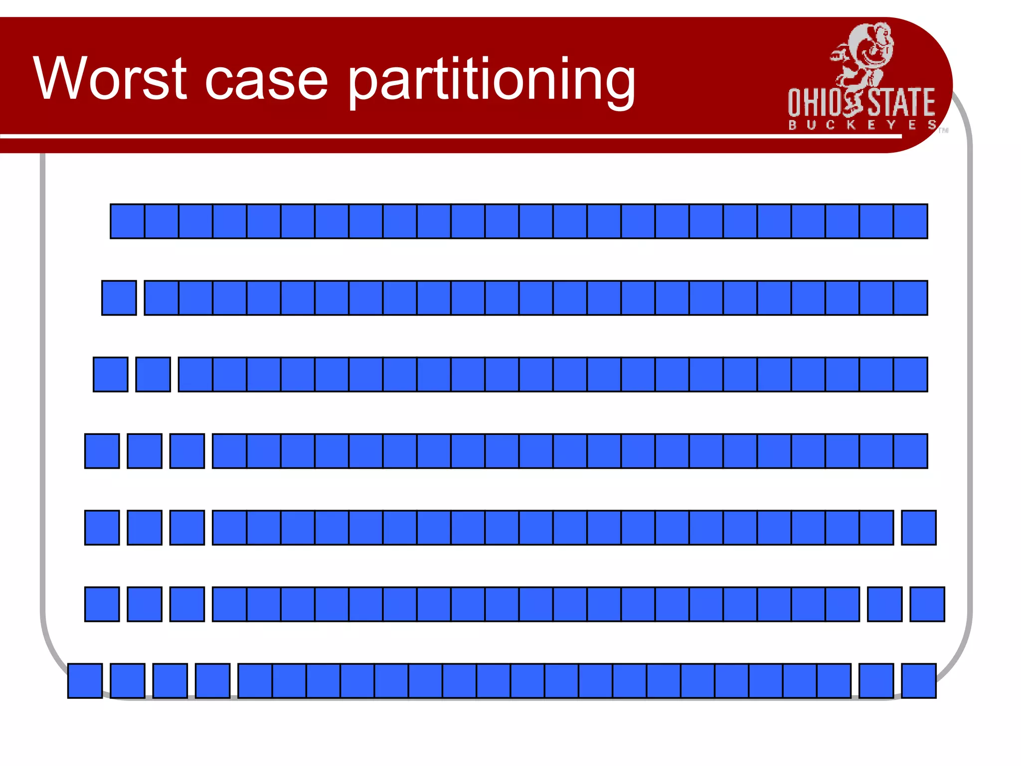
Worst case
 In the worst case, partitioning always
divides the size n array into these three
parts:
 A length one part, containing the pivot itself
 A length zero part, and
 A length n-1 part, containing everything else
 We don’t recur on the zero-length part
 Recurring on the length n-1 part requires
(in the worst case) recurring to depth n-1
Worst case partitioning
Worst case for quicksort
 In the worst case, recursion may be n levels deep
(for an array of size n)
 But the partitioning work done at each level is still n
 O(n) * O(n) = O(n2)
 So worst case for Quicksort is O(n2)
 When does this happen?
 There are many arrangements that could make this
happen
 Here are two common cases:
 When the array is already sorted
 When the array is inversely sorted (sorted in the opposite
order)
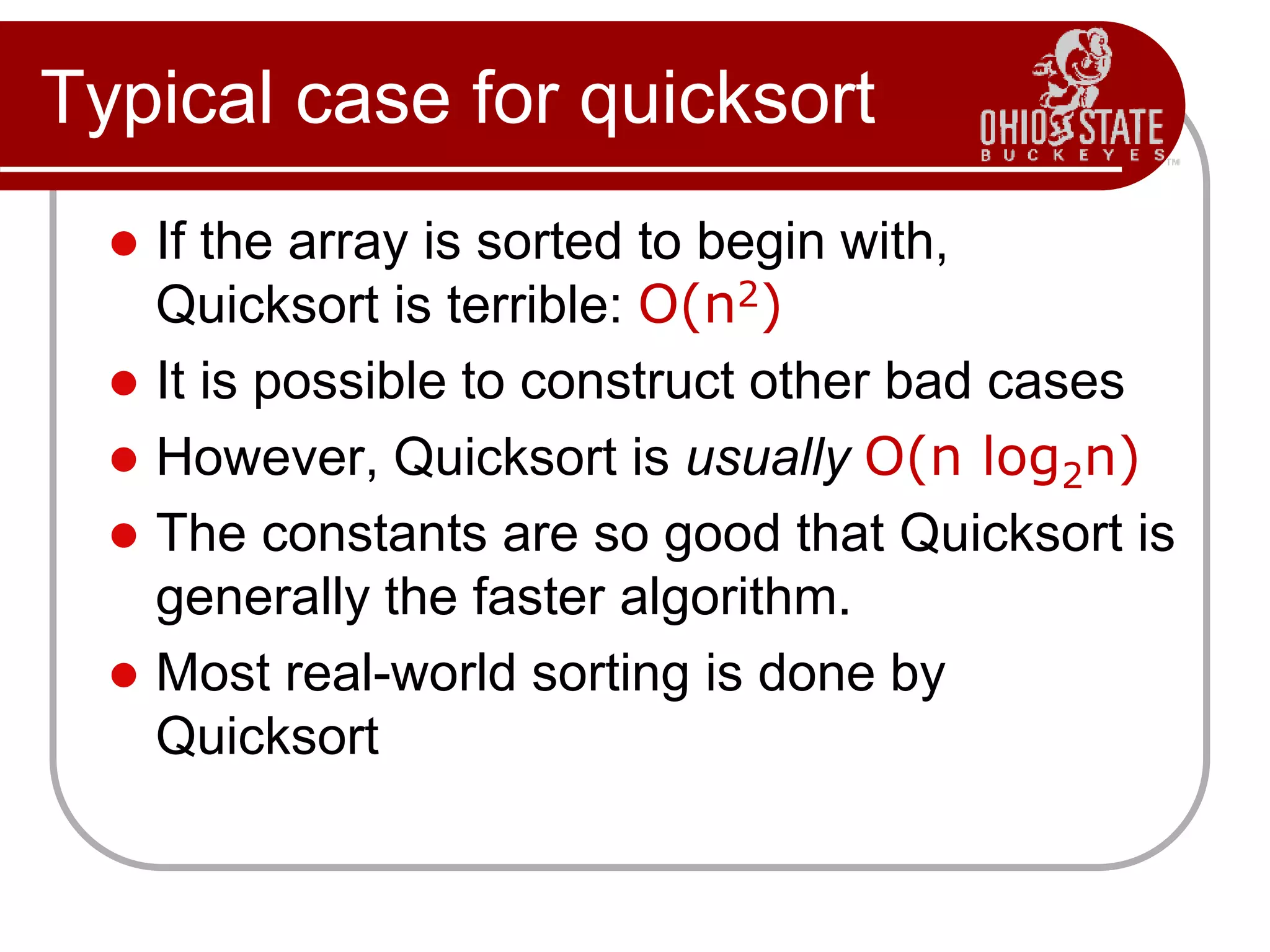
Typical case for quicksort
 If the array is sorted to begin with,
Quicksort is terrible: O(n2)
 It is possible to construct other bad cases
 However, Quicksort is usually O(n log2n)
 The constants are so good that Quicksort is
generally the faster algorithm.
 Most real-world sorting is done by
Quicksort
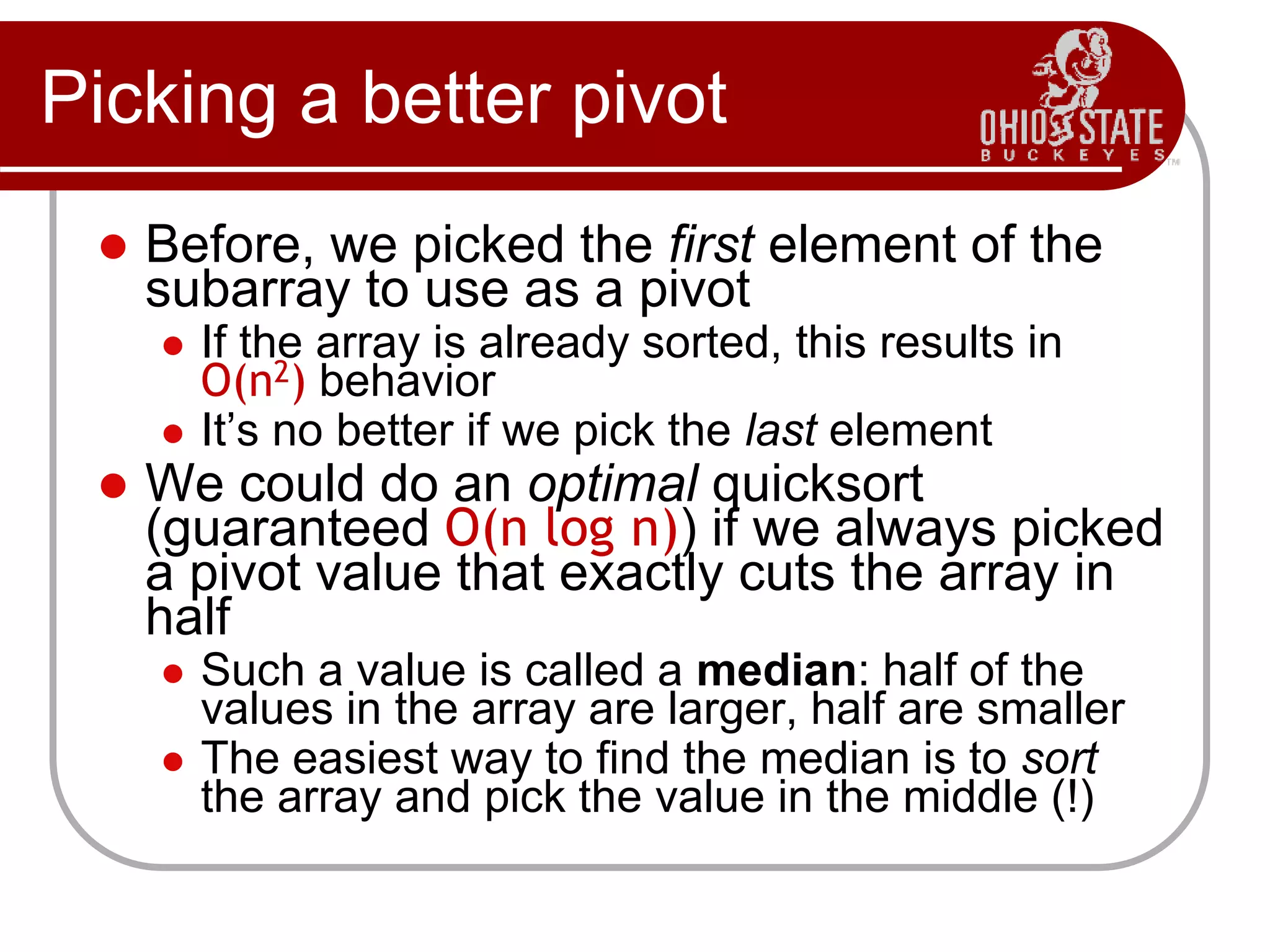
Picking a better pivot
 Before, we picked the first element of the
subarray to use as a pivot
 If the array is already sorted, this results in
O(n2) behavior
 It’s no better if we pick the last element
 We could do an optimal quicksort
(guaranteed O(n log n)) if we always picked
a pivot value that exactly cuts the array in
half
 Such a value is called a median: half of the
values in the array are larger, half are smaller
 The easiest way to find the median is to sort
the array and pick the value in the middle (!)
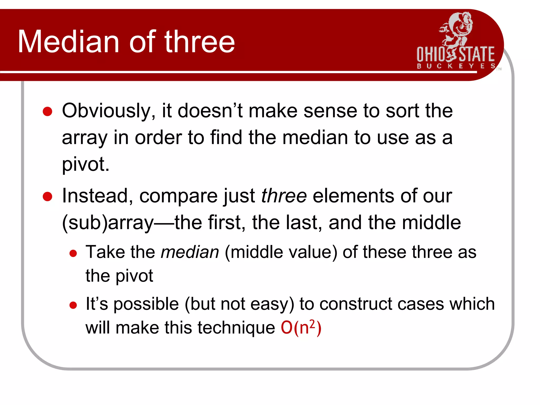
Median of three
 Obviously, it doesn’t make sense to sort the
array in order to find the median to use as a
pivot.
 Instead, compare just three elements of our
(sub)array—the first, the last, and the middle
 Take the median (middle value) of these three as
the pivot
 It’s possible (but not easy) to construct cases which
will make this technique O(n2)
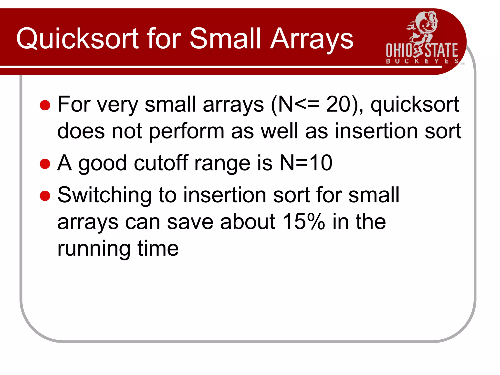
Quicksort for Small Arrays
 For very small arrays (N<= 20), quicksort
does not perform as well as insertion sort
 A good cutoff range is N=10
 Switching to insertion sort for small
arrays can save about 15% in the
running time
Mergesort vs Quicksort
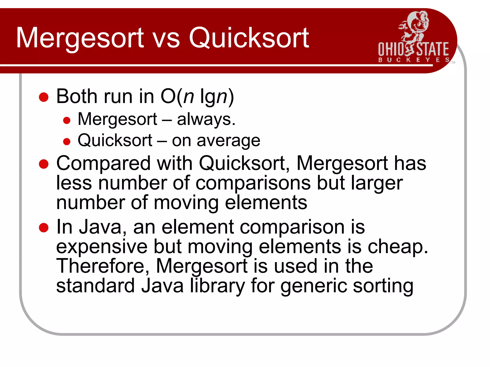
 Both run in O(n lgn)
 Mergesort – always.
 Quicksort – on average
 Compared with Quicksort, Mergesort has
less number of comparisons but larger
number of moving elements
 In Java, an element comparison is
expensive but moving elements is cheap.
Therefore, Mergesort is used in the
standard Java library for generic sorting
Mergesort vs Quicksort
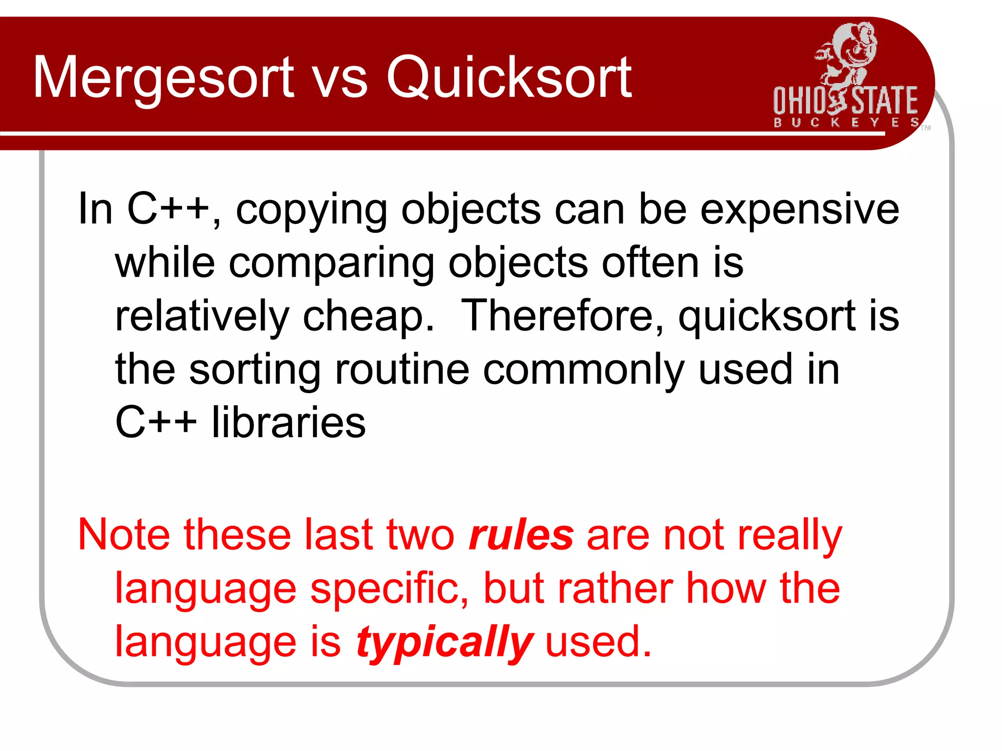
In C++, copying objects can be expensive
while comparing objects often is
relatively cheap. Therefore, quicksort is
the sorting routine commonly used in
C++ libraries
Note these last two rules are not really
language specific, but rather how the
language is typically used.

CSE680-07QuickSort.pptx

  • 1.
  • 2.
    Sorting Review  InsertionSort  T(n) = Q(n2)  In-place  Merge Sort  T(n) = Q(n lg(n))  Not in-place  Selection Sort (from homework)  T(n) = Q(n2)  In-place  Heap Sort  T(n) = Q(n lg(n))  In-place Seems pretty good. Can we do better?
  • 3.
    Sorting  Assumptions 1. Noknowledge of the keys or numbers we are sorting on. 2. Each key supports a comparison interface or operator. 3. Sorting entire records, as opposed to numbers, is an implementation detail. 4. Each key is unique (just for convenience). Comparison Sorting
  • 4.
    Comparison Sorting  Givena set of n values, there can be n! permutations of these values.  So if we look at the behavior of the sorting algorithm over all possible n! inputs we can determine the worst-case complexity of the algorithm.
  • 5.
    Decision Tree  Decisiontree model  Full binary tree  A proper binary tree (or 2-tree) is a tree in which every node other than the leaves has two children  Internal node represents a comparison.  Ignore control, movement, and all other operations, just see comparison  Each leaf represents one possible result (a permutation of the elements in sorted order).  The height of the tree (i.e., longest path) is the lower bound.
  • 6.
    Decision Tree Model 2:3 1:2 2:3 1:3 1:3 <1,2,3> <1,3,2><3,1,2> <2,1,3> <2,3,1> <3,2,1>     > > > > > Internal node i:j indicates comparison between ai and aj. suppose three elements < a1, a2, a3> with instance <6,8,5> Leaf node <(1), (2), (3)> indicates ordering a(1) a(2) a(3). Path of bold lines indicates sorting path for <6,8,5>. There are total 3!=6 possible permutations (paths). 
  • 7.
    Decision Tree Model The longest path is the worst case number of comparisons. The length of the longest path is the height of the decision tree.  Theorem 8.1: Any comparison sort algorithm requires (nlg n) comparisons in the worst case.  Proof:  Suppose height of a decision tree is h, and number of paths (i,e,, permutations) is n!.  Since a binary tree of height h has at most 2h leaves,  n!  2h , so h  lg (n!)  (nlg n) (By equation 3.18).  That is to say: any comparison sort in the worst case needs at least nlg n comparisons.
  • 8.
    QuickSort Design  Followsthe divide-and-conquer paradigm.  Divide: Partition (separate) the array A[p..r] into two (possibly empty) subarrays A[p..q–1] and A[q+1..r].  Each element in A[p..q–1] < A[q].  A[q] < each element in A[q+1..r].  Index q is computed as part of the partitioning procedure.  Conquer: Sort the two subarrays by recursive calls to quicksort.  Combine: The subarrays are sorted in place – no work is needed to combine them.  How do the divide and combine steps of quicksort compare with those of merge sort?
  • 9.
    Pseudocode Quicksort(A, p, r) ifp < r then q := Partition(A, p, r); Quicksort(A, p, q – 1); Quicksort(A, q + 1, r) Partition(A, p, r) x, i := A[r], p – 1; for j := p to r – 1 do if A[j]  x then i := i + 1; A[i]  A[j] A[i + 1]  A[r]; return i + 1 5 A[p..r] A[p..q – 1] A[q+1..r]  5  5 Partition 5
  • 10.
    Example p r initially: 25 8 3 9 4 1 7 10 6 note: pivot (x) = 6 i j next iteration: 2 5 8 3 9 4 1 7 10 6 i j next iteration: 2 5 8 3 9 4 1 7 10 6 i j next iteration: 2 5 8 3 9 4 1 7 10 6 i j next iteration: 2 5 3 8 9 4 1 7 10 6 i j Partition(A, p, r) x, i := A[r], p – 1; for j := p to r – 1 do if A[j]  x then i := i + 1; A[i]  A[j] A[i + 1]  A[r]; return i + 1
  • 11.
    Example (Continued) next iteration:2 5 3 8 9 4 1 7 10 6 i j next iteration: 2 5 3 8 9 4 1 7 10 6 i j next iteration: 2 5 3 4 9 8 1 7 10 6 i j next iteration: 2 5 3 4 1 8 9 7 10 6 i j next iteration: 2 5 3 4 1 8 9 7 10 6 i j next iteration: 2 5 3 4 1 8 9 7 10 6 i j after final swap: 2 5 3 4 1 6 9 7 10 8 i j Partition(A, p, r) x, i := A[r], p – 1; for j := p to r – 1 do if A[j]  x then i := i + 1; A[i]  A[j] A[i + 1]  A[r]; return i + 1
  • 12.
    Partitioning  Select thelast element A[r] in the subarray A[p..r] as the pivot – the element around which to partition.  As the procedure executes, the array is partitioned into four (possibly empty) regions. 1. A[p..i ] — All entries in this region are < pivot. 2. A[i+1..j – 1] — All entries in this region are > pivot. 3. A[r] = pivot. 4. A[j..r – 1] — Not known how they compare to pivot.  The above hold before each iteration of the for loop, and constitute a loop invariant. (4 is not part of the loopi.)
  • 13.
    Correctness of Partition Use loop invariant.  Initialization:  Before first iteration  A[p..i] and A[i+1..j – 1] are empty – Conds. 1 and 2 are satisfied (trivially).  r is the index of the pivot  Cond. 3 is satisfied.  Maintenance:  Case 1: A[j] > x  Increment j only.  Loop Invariant is maintained. Partition(A, p, r) x, i := A[r], p – 1; for j := p to r – 1 do if A[j]  x then i := i + 1; A[i]  A[j] A[i + 1]  A[r]; return i + 1
  • 14.
    Correctness of Partition >xx p i j r  x > x x p i j r  x > x Case 1:
  • 15.
    Correctness of Partition Case 2: A[j]  x  Increment i  Swap A[i] and A[j]  Condition 1 is maintained.  Increment j  Condition 2 is maintained.  A[r] is unaltered.  Condition 3 is maintained.  x x p i j r  x > x  x > x x p i j r
  • 16.
    Correctness of Partition Termination:  When the loop terminates, j = r, so all elements in A are partitioned into one of the three cases:  A[p..i]  pivot  A[i+1..j – 1] > pivot  A[r] = pivot  The last two lines swap A[i+1] and A[r].  Pivot moves from the end of the array to between the two subarrays.  Thus, procedure partition correctly performs the divide step.
  • 17.
    Complexity of Partition PartitionTime(n) is given by the number of iterations in the for loop.  Q(n) : n = r – p + 1. Partition(A, p, r) x, i := A[r], p – 1; for j := p to r – 1 do if A[j]  x then i := i + 1; A[i]  A[j] A[i + 1]  A[r]; return i + 1
  • 18.
    Quicksort Overview  Tosort a[left...right]: 1. if left < right: 1.1. Partition a[left...right] such that: all a[left...p-1] are less than a[p], and all a[p+1...right] are >= a[p] 1.2. Quicksort a[left...p-1] 1.3. Quicksort a[p+1...right] 2. Terminate
  • 19.
    Partitioning in Quicksort A key step in the Quicksort algorithm is partitioning the array  We choose some (any) number p in the array to use as a pivot  We partition the array into three parts: p numbers less than p numbers greater than or equal to p p
  • 20.
    Alternative Partitioning  Choosean array value (say, the first) to use as the pivot  Starting from the left end, find the first element that is greater than or equal to the pivot  Searching backward from the right end, find the first element that is less than the pivot  Interchange (swap) these two elements  Repeat, searching from where we left off, until done
  • 21.
    Alternative Partitioning  Topartition a[left...right]: 1. Set pivot = a[left], l = left + 1, r = right; 2. while l < r, do 2.1. while l < right & a[l] < pivot , set l = l + 1 2.2. while r > left & a[r] >= pivot , set r = r - 1 2.3. if l < r, swap a[l] and a[r] 3. Set a[left] = a[r], a[r] = pivot 4. Terminate
  • 22.
    Example of partitioning choose pivot: 4 3 6 9 2 4 3 1 2 1 8 9 3 5 6  search: 4 3 6 9 2 4 3 1 2 1 8 9 3 5 6  swap: 4 3 3 9 2 4 3 1 2 1 8 9 6 5 6  search: 4 3 3 9 2 4 3 1 2 1 8 9 6 5 6  swap: 4 3 3 1 2 4 3 1 2 9 8 9 6 5 6  search: 4 3 3 1 2 4 3 1 2 9 8 9 6 5 6  swap: 4 3 3 1 2 2 3 1 4 9 8 9 6 5 6  search: 4 3 3 1 2 2 3 1 4 9 8 9 6 5 6  swap with pivot: 1 3 3 1 2 2 3 4 4 9 8 9 6 5 6
  • 23.
    Partition Implementation (Java) staticint Partition(int[] a, int left, int right) { int p = a[left], l = left + 1, r = right; while (l < r) { while (l < right && a[l] < p) l++; while (r > left && a[r] >= p) r--; if (l < r) { int temp = a[l]; a[l] = a[r]; a[r] = temp; } } a[left] = a[r]; a[r] = p; return r; }
  • 24.
    Quicksort Implementation (Java) staticvoid Quicksort(int[] array, int left, int right) { if (left < right) { int p = Partition(array, left, right); Quicksort(array, left, p - 1); Quicksort(array, p + 1, right); } }
  • 25.
    Analysis of quicksort—bestcase  Suppose each partition operation divides the array almost exactly in half  Then the depth of the recursion in log2n  Because that’s how many times we can halve n  We note that  Each partition is linear over its subarray  All the partitions at one level cover the array
  • 26.
  • 27.
    Best Case Analysis We cut the array size in half each time  So the depth of the recursion in log2n  At each level of the recursion, all the partitions at that level do work that is linear in n  O(log2n) * O(n) = O(n log2n)  Hence in the best case, quicksort has time complexity O(n log2n)  What about the worst case?
  • 28.
    Worst case  Inthe worst case, partitioning always divides the size n array into these three parts:  A length one part, containing the pivot itself  A length zero part, and  A length n-1 part, containing everything else  We don’t recur on the zero-length part  Recurring on the length n-1 part requires (in the worst case) recurring to depth n-1
  • 29.
  • 30.
    Worst case forquicksort  In the worst case, recursion may be n levels deep (for an array of size n)  But the partitioning work done at each level is still n  O(n) * O(n) = O(n2)  So worst case for Quicksort is O(n2)  When does this happen?  There are many arrangements that could make this happen  Here are two common cases:  When the array is already sorted  When the array is inversely sorted (sorted in the opposite order)
  • 31.
    Typical case forquicksort  If the array is sorted to begin with, Quicksort is terrible: O(n2)  It is possible to construct other bad cases  However, Quicksort is usually O(n log2n)  The constants are so good that Quicksort is generally the faster algorithm.  Most real-world sorting is done by Quicksort
  • 32.
    Picking a betterpivot  Before, we picked the first element of the subarray to use as a pivot  If the array is already sorted, this results in O(n2) behavior  It’s no better if we pick the last element  We could do an optimal quicksort (guaranteed O(n log n)) if we always picked a pivot value that exactly cuts the array in half  Such a value is called a median: half of the values in the array are larger, half are smaller  The easiest way to find the median is to sort the array and pick the value in the middle (!)
  • 33.
    Median of three Obviously, it doesn’t make sense to sort the array in order to find the median to use as a pivot.  Instead, compare just three elements of our (sub)array—the first, the last, and the middle  Take the median (middle value) of these three as the pivot  It’s possible (but not easy) to construct cases which will make this technique O(n2)
  • 34.
    Quicksort for SmallArrays  For very small arrays (N<= 20), quicksort does not perform as well as insertion sort  A good cutoff range is N=10  Switching to insertion sort for small arrays can save about 15% in the running time
  • 35.
    Mergesort vs Quicksort Both run in O(n lgn)  Mergesort – always.  Quicksort – on average  Compared with Quicksort, Mergesort has less number of comparisons but larger number of moving elements  In Java, an element comparison is expensive but moving elements is cheap. Therefore, Mergesort is used in the standard Java library for generic sorting
  • 36.
    Mergesort vs Quicksort InC++, copying objects can be expensive while comparing objects often is relatively cheap. Therefore, quicksort is the sorting routine commonly used in C++ libraries Note these last two rules are not really language specific, but rather how the language is typically used.