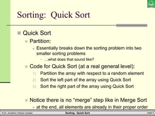
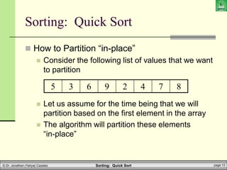
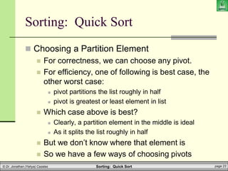
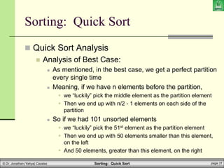
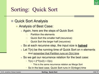
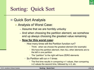
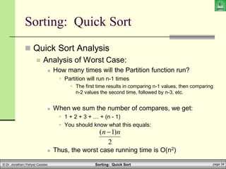
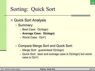
This document discusses quick sort, one of the most common sorting algorithms. Quick sort uses two main ideas - partitioning and recursion. It works by partitioning an array around a pivot element, and then recursively sorting the subarrays on each side of the pivot. In the best case, where the pivot always partitions the array in half, quick sort runs in O(n log n) time. However, its performance depends on how well it can partition the array on each iteration. The document provides pseudocode for quick sort and discusses strategies for choosing a good pivot element to improve its average runtime.

![Sorting: Quick Sort page 9
© Dr. Jonathan (Yahya) Cazalas
Sorting: Quick Sort
The idea of “in place”
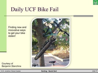
In Computer Science, an “in-place” algorithm is
one where the output usually overwrites the input
There is more detail, but for our purposes, we stop with
that
Example:
Say we wanted to reverse an array of n items
Here is a simple way to do that:
method reverse(a[0..n]) {
allocate b[0..n]
for i from 0 to n
b[n - i] = a[i]
return b
}](https://image.slidesharecdn.com/cpcs20423quicksort-210408140321/85/quick_sort-9-320.jpg)
![Sorting: Quick Sort page 10
© Dr. Jonathan (Yahya) Cazalas
Sorting: Quick Sort
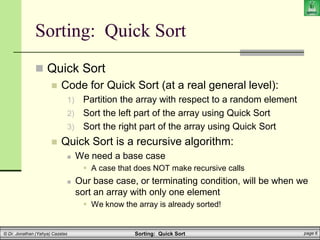
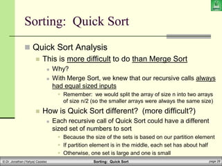
The idea of “in place”
Example:
Say we wanted to reverse an array of n items
Here is a simple way to do that:
Unfortunately, this method requires O(n) extra space to
create the array b
And allocation can be a slow operation
method reverse(a[0..n]) {
allocate b[0..n]
for i from 0 to n
b[n - i] = a[i]
return b
}](https://image.slidesharecdn.com/cpcs20423quicksort-210408140321/85/quick_sort-10-320.jpg)
![Sorting: Quick Sort page 11
© Dr. Jonathan (Yahya) Cazalas
Sorting: Quick Sort
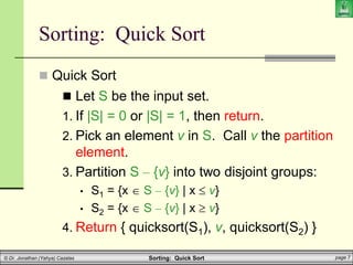
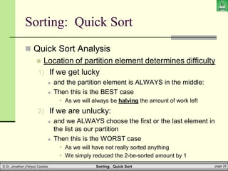
The idea of “in place”
Example:
Say we wanted to reverse an array of n items
If we no longer need the original array a
We can overwrite it using the following in-place algorithm
Many Sorting algorithms are in-place algorithms
Quick sort is NOT an in-place algorithm
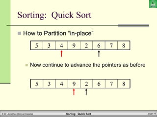
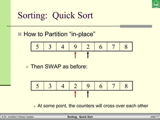
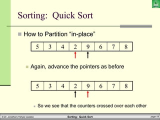
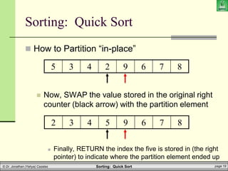
BUT, the Partition algorithm can be in-place
method reverse-in-place(a[0..n])
for i from 0 to floor(n/2)
swap(a[i], a[n-i])](https://image.slidesharecdn.com/cpcs20423quicksort-210408140321/85/quick_sort-11-320.jpg)
![Sorting: Quick Sort page 20
© Dr. Jonathan (Yahya) Cazalas
Sorting: Quick Sort
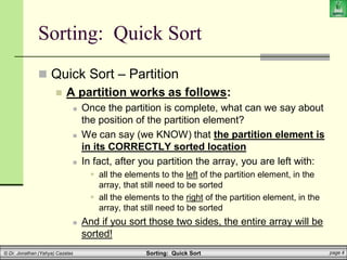
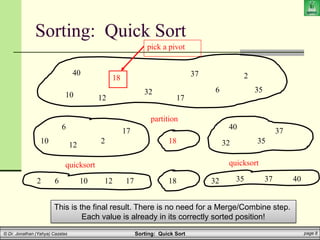
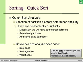
Partition Code
public int partition(int vals[], int low, int high) {
int temp, randomIndex;
int pivotIdx; // index of the pivot element
// A base case that should never really occur.
if (low == high) return low;
// Pick a random partition element and swap it into index low.
randomIndex = low + (int)(Math.random()*(high-low+1));
temp = vals[randomIndex];
vals[randomIndex] = vals[low];
vals[low] = temp;
// Store the index of the partition element.
pivotIdx = low; // set pivotIdx to the position index of “low”
// Update our low pointer.
low++;](https://image.slidesharecdn.com/cpcs20423quicksort-210408140321/85/quick_sort-20-320.jpg)
![Sorting: Quick Sort page 21
© Dr. Jonathan (Yahya) Cazalas
Sorting: Quick Sort
Partition Code
// Run Partition so long as low and high counters don't cross.
while (low <= high) {
// Move the low pointer forwards.
while (low <= high && vals[low] <= vals[pivot]) low++;
// Move the high pointer backwards.
while (high >= low && vals[high] > vals[pivot]) high--;
// Now swap the values at those two pointers.
if (low < high)
swap(vals, low, high);
}
// Swap the partition element into it's correct location.
swap(vals, pivotIdx, high);
return high; // Return the FINAL index of the partition element.
}](https://image.slidesharecdn.com/cpcs20423quicksort-210408140321/85/quick_sort-21-320.jpg)
![Sorting: Quick Sort page 22
© Dr. Jonathan (Yahya) Cazalas
Sorting: Quick Sort
Quick Sort Code
public void quickSort(int numbers[], int low, int high) {
// Only have to sort if we are sorting more than one number
if (low < high) {
// Partition the elements
// Parition function returns the index of the
// partition element. Saved into “pivot”.
int pivotIdx = partition(numbers, low, high);
// Recursively Quick Sort the left side
quickSort(numbers, low, pivotIdx-1);
// Recursively Quick Sort the right side
quickSort(numbers, pivotIdx+1, high);
}
}](https://image.slidesharecdn.com/cpcs20423quicksort-210408140321/85/quick_sort-22-320.jpg)

![ppt daaa[1].pptxdaaaaaaaaaaaaaaaaaaaaaaaaaaaaaaaaa](https://cdn.slidesharecdn.com/ss_thumbnails/pptdaaa1-251211161628-1cb28a51-thumbnail.jpg?width=640&height=640&fit=bounds)


![UNIT V Searching Sorting Hashing Techniques [Autosaved].pptx](https://cdn.slidesharecdn.com/ss_thumbnails/unitvsearchingsortinghashingtechniquesautosaved-241126054304-95a69c51-thumbnail.jpg?width=640&height=640&fit=bounds)

![UNIT V Searching Sorting Hashing Techniques [Autosaved].pptx](https://cdn.slidesharecdn.com/ss_thumbnails/unitvsearchingsortinghashingtechniquesautosaved-241014040608-74caa0f6-thumbnail.jpg?width=640&height=640&fit=bounds)