Downloaded 776 times
![Quick Sort Divide: Partition the array into two sub-arrays A[p . . q-1] and A[q+1 . . r] such that each element of A[p . . q-1] is less than or equal to A[q], which in turn less than or equal to each element of A[q+1 . . r]](https://image.slidesharecdn.com/quicksortppt2114/85/Algorithm-Quick-Sort-1-320.jpg)
![Quick Sort Divide: Partition the array into two sub-arrays A[p . . q-1] and A[q+1 . . r] such that each element of A[p . . q-1] is less than or equal to A[q], which in turn less than or equal to each element of A[q+1 . . r]](https://image.slidesharecdn.com/quicksortppt2114/75/Algorithm-Quick-Sort-1-2048.jpg)
![Quick Sort Conquer: Sort the two sub-arrays A[p . . q-1] and A[q+1 . . r] by recursive calls to quick sort.](https://image.slidesharecdn.com/quicksortppt2114/85/Algorithm-Quick-Sort-2-320.jpg)
![Quick Sort PARTITION(A, p, r) x A[r] i p-1](https://image.slidesharecdn.com/quicksortppt2114/85/Algorithm-Quick-Sort-5-320.jpg)
![Quick Sort for j p to r-1 do if A[j] <= x then i i+1 exchange A[i] A[j] exchange A[i+1] A[r] return i+1](https://image.slidesharecdn.com/quicksortppt2114/85/Algorithm-Quick-Sort-6-320.jpg)
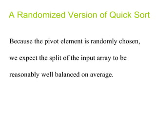
![A Randomized Version of Quick Sort Instead of always using A[r] as the pivot, we will use a randomly chosen element from the sub-array A[p..r].](https://image.slidesharecdn.com/quicksortppt2114/85/Algorithm-Quick-Sort-30-320.jpg)
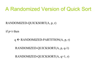
![A Randomized Version of Quick Sort RANDOMIZED-PARTITION(A, p, r) i RANDOM(p, r) exchange A[r] A[i] return PARTITION(A, p, r)](https://image.slidesharecdn.com/quicksortppt2114/85/Algorithm-Quick-Sort-32-320.jpg)

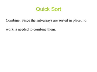
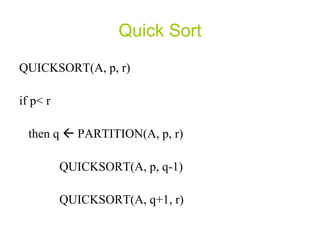
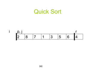
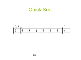
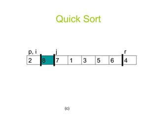
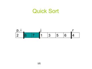
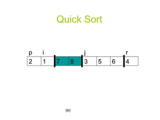
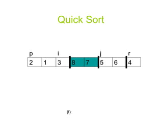
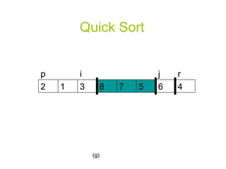
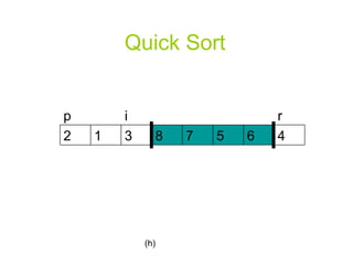
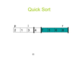
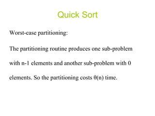
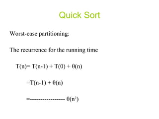
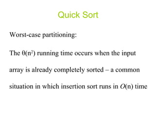
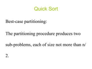
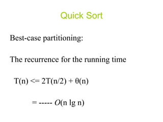
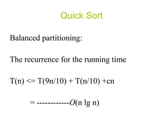
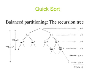
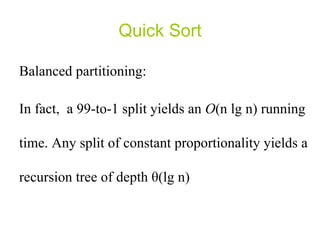
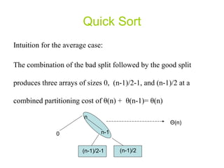
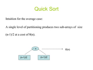
The document describes the quicksort algorithm. Quicksort works by: 1) Partitioning the array around a pivot element into two sub-arrays of less than or equal and greater than elements. 2) Recursively sorting the two sub-arrays. 3) Combining the now sorted sub-arrays. In the average case, quicksort runs in O(n log n) time due to balanced partitions at each recursion level. However, in the worst case of an already sorted input, it runs in O(n^2) time due to highly unbalanced partitions. A randomized version of quicksort chooses pivots randomly to avoid worst case behavior.


![ppt daaa[1].pptxdaaaaaaaaaaaaaaaaaaaaaaaaaaaaaaaaa](https://cdn.slidesharecdn.com/ss_thumbnails/pptdaaa1-251211161628-1cb28a51-thumbnail.jpg?width=640&height=640&fit=bounds)