
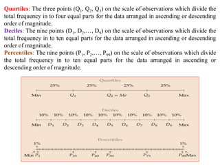

![PARTITIONS VALUES FOR GROUPED DATA: Continuous frequency distribution
In the case of Continuous frequency distribution the computation of partitions values
involves the following steps:
1. Arranged the data in ascending order of magnitude (if not arranged).
2. Find the less than type cumulative frequencies (c.f.).
3. Convert the classes into exclusive form if given otherwise
4. Calculate the partitions values using following formulae.
Where, x = 1, 2, 3
C
4
N
x
f
i
L
Q
Quartile 1
x
Where
L1 = lower limit of quartile class
N = total number of observations i.e. sum of frequencies
C = cumulative frequency of the class previous the quartile class
f = frequency of quartile class
i = class width i.e. Magnitude of quartile class
Quartile class: The class which contains [( x N)/4 ]th term.](https://image.slidesharecdn.com/topic4quartiledecilepercentile-240117104641-c74531c9/85/Statistical-Methods-Quartile-Decile-Percentile-pptx-10-320.jpg)
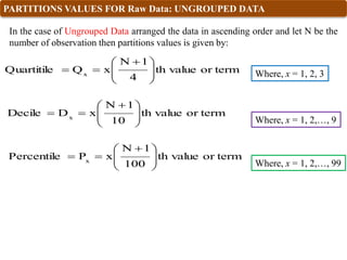
![Where, x = 1, 2,…,9
C
10
N
x
f
i
L
D
Decile 1
x
Where
L1 = lower limit of Decile class
N = total number of observations i.e. sum of frequencies
C = cumulative frequency of the class previous the Decile class
f = frequency of Decile class
i = class width i.e. Magnitude of Decile class
Decile class: The class which contains [( x N)/10 ]th term.
Where, x = 1, 2,…,99
C
100
N
x
f
i
L
P
Percentile 1
x
Where
L1 = lower limit of Percentile class
N = total number of observations i.e. sum of frequencies
C = cumulative frequency of the class previous the Percentile class
f = frequency of Percentile class
i = class width i.e. Magnitude of Percentile class
Percentile class: The class which contains [( x N)/100 ]th term.](https://image.slidesharecdn.com/topic4quartiledecilepercentile-240117104641-c74531c9/85/Statistical-Methods-Quartile-Decile-Percentile-pptx-11-320.jpg)
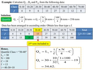
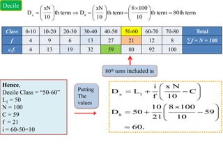
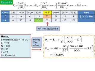


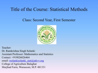
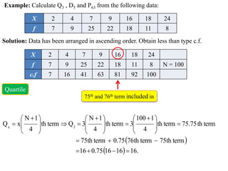
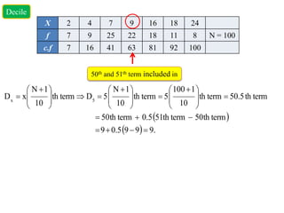
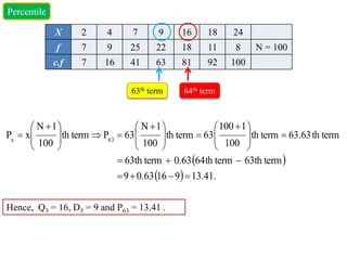
This document provides information about calculating quartiles, deciles, and percentiles from grouped and ungrouped data. It defines quartiles, deciles, and percentiles as points that divide the total frequency of data into four, ten, and one hundred equal parts, respectively. Formulas are provided to calculate the first, second, third, etc. quartile, decile, and percentile values based on the cumulative frequency of data arranged in ascending or descending order. An example calculation is shown for finding the first quartile, eighth decile, and 56th percentile from a grouped frequency distribution.