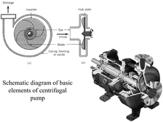
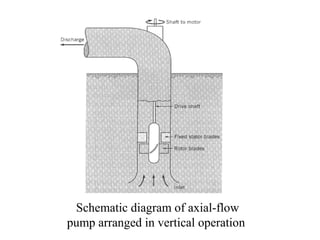
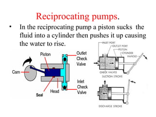
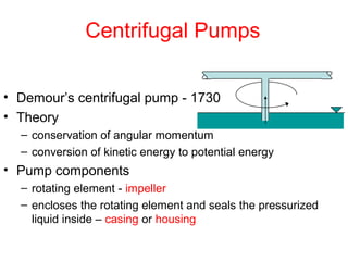
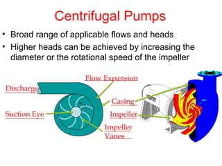
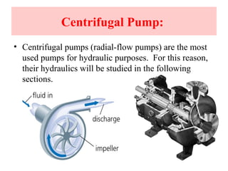
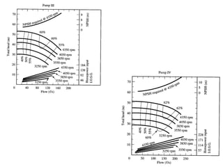
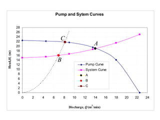
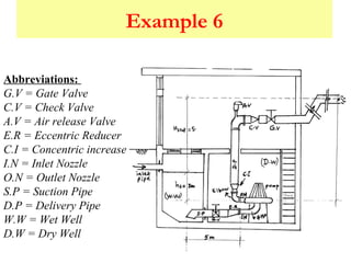
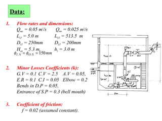
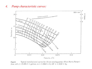
SlideShare a Scribd company logo
Water Pumps
The Islamic University of Gaza
Faculty of Engineering
Civil Engineering Department
Hydraulics - ECIV 3322
Chapter 5Chapter 5

Definition
• Water pumps are devices designed to convert
mechanical energy to hydraulic energy.
• They are used to move water from lower
points to higher points with a required
discharge and pressure head.
• This chapter will deal with the basic hydraulic
concepts of water pumps
Pump Classification
• Turbo-hydraulic (kinetic) pumps
Centrifugal pumps (radial-flow pumps)
Propeller pumps (axial-flow pumps)
Jet pumps (mixed-flow pumps)
• Positive-displacement pumps
Screw pumps
Reciprocating pumps
• This classification is based on the
way by which the water leaves the
rotating part of the pump.
• In radial-flow pump the water
leaves the impeller in radial
direction,
• while in the axial-flow pump the
water leaves the propeller in the
axial direction.
• In the mixed-flow pump the water
leaves the impeller in an inclined
direction having both radial and
axial components
Schematic diagram of basic
elements of centrifugal
pump
Schematic diagram of axial-flow
pump arranged in vertical operation
Screw pumps.
• In the screw pump a revolving shaft fitted with
blades rotates in an inclined trough and pushes the
water up the trough.
Reciprocating pumps.
• In the reciprocating pump a piston sucks the
fluid into a cylinder then pushes it up causing
the water to rise.
‫ه‬‫ه‬‫ه‬‫ه‬‫ه‬‫ه‬‫ه‬‫ه‬‫ه‬
‫ه‬‫ه‬‫ه‬‫ه‬
‫ه‬‫ه‬‫ه‬‫ه‬‫ه‬‫ه‬‫ه‬‫ه‬
Centrifugal Pumps
• Demour’s centrifugal pump - 1730
• Theory
– conservation of angular momentum
– conversion of kinetic energy to potential energy
• Pump components
– rotating element - impeller
– encloses the rotating element and seals the pressurized
liquid inside – casing or housing
Centrifugal Pumps
Impeller
Vanes
Casing
Suction Eye Impeller
Discharge
Flow Expansion
• Broad range of applicable flows and heads
• Higher heads can be achieved by increasing the
diameter or the rotational speed of the impeller
Centrifugal Pump:
• Centrifugal pumps (radial-flow pumps) are the most
used pumps for hydraulic purposes. For this reason,
their hydraulics will be studied in the following
sections.
Main Parts of Centrifugal Pumps
• which is the rotating part of
the centrifugal pump.
• It consists of a series of
backwards curved vanes
(blades).
• The impeller is driven by a
shaft which is connected to the
shaft of an electric motor.
1. Impeller:
Main Parts of Centrifugal Pumps
• Which is an air-tight
passage surrounding the
impeller
• designed to direct the
liquid to the impeller
and lead it away
• Volute casing. It is of
spiral type in which the
area of the flow
increases gradually.
2. Casing
3. Suction Pipe.
4. Delivery Pipe.
5. The Shaft: which is the bar by which the
power is transmitted from the motor drive to
the impeller.
6. The driving motor: which is responsible for
rotating the shaft. It can be mounted directly
on the pump, above it, or adjacent to it.
Note that a centrifugal pump can be
either submersible (wet) or dry.
Hydraulic Analysis of Pumps and Piping
Systems
• Pump can be placed in two possible position in
reference to the water levels in the reservoirs.
• We begin our study by defining all the
different terms used to describe the pump
performance in the piping system.
Hydraulic Analysis of Pumps and Piping Systems
Ht
hd
Hstat
hs
Hms
Hmd
Datum pump
center line
hfs
hfd
Case 1
Hstat
HmdHms
hd
Ht
hs
Datum pump
center line
hfd
hfs
Case 2
The following terms can be defined
• hs (static suction head): it is the difference in
elevation between the suction liquid level and the
centerline of the pump impeller.
• hd (static discharge head): it is the difference in
elevation between the discharge liquid level and
the centerline of the pump impeller.
• Hstat (static head): it is the difference (or sum) in
elevation between the static discharge and the
static suction heads: H h hstat d s= ±
• Hms (manometric suction head): it is the suction
gage reading (if a manometer is installed just at the
inlet of the pump, then Hms is the height to which
the water will rise in the manometer).
• Hmd (manometric discharge head): it is the
discharge gage reading (if a manometer is installed
just at the outlet of the pump, then Hmd is the height
to which the water will rise in the manometer).
• Hm (manometric head): it is the increase of
pressure head generated by the pump:
H H Hm md ms= ±
• Ht (total dynamic head): it is the total head
delivered by the pump:
H H
V
g
H
V
gt md
d
m s
s
= + − +
2 2
2 2
( )
H H
V
g
H
V
gt md
d
m s
s
= + + −
2 2
2 2
( )
Case 1
Case 2
Eq.(1)
Eq.(2)
• Ht can be written in another form as follows:
H h h hmd d f d md= + + ∑
H h h h
V
gms s f s ms
s
= − − −∑
2
2
H h h h
V
gms s f s ms
s
= + + +∑
2
2
Case 1
Case 2
H h h h
V
g
h h h
V
g
V
gt d f d md
d
s f s ms
s s
= + + ∑ + − − − − +∑








2 2 2
2 2 2
H h hstat d s= −
but
H H h h h h
V
gt stat f d md f s ms
d
= + + ∑ + + +∑
2
2
Substitute ino eq. (1)
Eq.(3)
Case 1
• Equation (3) can be applied to Case 2 with the
exception that : H h hstat d s= +
In the above equations; we define:
hfs : is the friction losses in the suction pipe.
hfd : is the friction losses in the discharge (delivery) pipe.
hms : is the minor losses in the suction pipe.
hmd: is the minor losses in the discharge (delivery) pipe.
• Bernoulli’s equation can also be applied to find Ht
H
P V
g
Z
P V
g
Zt
d d
d
s s
s= + + ± + +





γ γ
2 2
2 2
Eq.(4)
Pump Efficiency
η
γ
p
o
i
t
i
Power output
Power input
P
P
Q H
P
= = =
P
Q H
i
t
p
=
γ
η
or
Which is the power input delivered from the motor to the
impeller of the pump.
Motor efficiency : ηm
ηm
i
m
P
P
=
P
P
m
i
m
=
η
which is the power input delivered to the motor.
ηo
η η ηo p m=
ηo
o
m
P
P
=
Overall efficiency of the motor-pump system:
Cavitation of Pumps and NPSH
• In general, cavitation occurs when the liquid pressure
at a given location is reduced to the vapor pressure of
the liquid.
• For a piping system that includes a pump, cavitation
occurs when the absolute pressure at the inlet falls
below the vapor pressure of the water.
• This phenomenon may occur at the inlet to a pump and
on the impeller blades, particularly if the pump is
mounted above the level in the suction reservoir.
• Under this condition, vapor bubbles form (water
starts to boil) at the impeller inlet and when these
bubbles are carried into a zone of higher pressure,
they collapse abruptly and hit the vanes of the
impeller (near the tips of the impeller vanes).
causing:
• Damage to the pump (pump impeller)
• Violet vibrations (and noise).
• Reduce pump capacity.
• Reduce pump efficiency
• To avoid cavitation, the pressure head at the inlet should not fall
below a certain minimum which is influenced by the further
reduction in pressure within the pump impeller.
• To accomplish this, we use the difference between the total head
at the inlet , and the water vapor pressure head
g
VP ss
2
2
+
γ
γ
vaporP
How we avoid Cavitation ??
Where we take the datum through the centerline of the pump
impeller inlet (eye). This difference is called the Net Positive
Suction Head (NPSH), so that
NPSH
P V
g
Ps s vapor
= + −
γ γ
2
2
There are two values of NPSH of interest. The first is the required NPSH,
denoted (NPSH)R , that must be maintained or exceeded so that cavitation
will not occur and usually determined experimentally and provided by the
manufacturer.
The second value for NPSH of concern is the available NPSH, denoted
(NPSH)A , which represents the head that actually occurs for the particular
piping system. This value can be determined experimentally, or calculated if
the system parameters are known.
How we avoid Cavitation ??
• For proper pump operation (no cavitation) :
(NPSH)A > (NPSH)R
Determination of
(NPSH)A
datum
hs
applying the energy equation between
point (1) and (2), datum at pump
center line
γγ
γγγγ
γγ
γγ
Vapor
LS
atm
A
Vapor
LS
atmVaporSS
LS
atmSS
L
SS
S
atm
P
hh
P
NPSH
P
hh
PP
g
VP
hh
P
g
VP
h
g
VP
h
P
−−−=
−−−=−+
−−=+
++=−
∑
∑
∑
∑
)(
2
2
2
2
2
2
( )NPSH h h h
P P
A s f s m s
atm vapor
= − − + −∑
γ γ
Note that (+) is used if hs is above the pump centerline (datum).
2
2
o
/335.2
/14.10
20Tat
mkNP
mkNP
Vapor
atm
=
=
=
Thoma’s cavitation constant
The cavitation constant: is the ratio of (NPSH)R
to
the total dynamic head (Ht
) is known as the Thoma’s
cavitation constant ( )σ
σ =
( )NPSH
H
R
t
Note: If the cavitation constant is given, we can find the
maximum allowable elevation of the pump inlet (eye)
above the surface of the supply (suction) reservoir.
Selection of A Pump
It has been seen that the efficiency of a pump depends on the discharge,
head, and power requirement of the pump. The approximate ranges of
application of each type of pump are indicated in the following Figure.
Selection of A Pump
• In selecting a particular pump for a given system:
• The design conditions are specified and a pump is selected
for the range of applications.
• A system characteristic curve (H-Q) is then prepared.
• The H-Q curve is then matched to the pump characteristics
chart which is provided by the manufacturer.
• The matching point (operating point) indicates the actual
working conditions.
System Characteristic Curve
The total head, Ht , that the pump delivers includes the
elevation head and the head losses incurred in the system. The
friction loss and other minor losses in the pipeline depend on the
velocity of the water in the pipe, and hence the total head loss
can be related to the discharge rate
For a given pipeline system (including a pump or a group of
pumps), a unique system head-capacity (H-Q) curve can be
plotted. This curve is usually referred to as a system
characteristic curve or simply system curve. It is a graphic
representation of the system head and is developed by plotting
the total head, over a range of flow rates starting from zero to
the maximum expected value of Q.
∑+= Lstatt hHH
)()( 12 QfnzzH p +−=
system
system
curve
0
20
40
60
80
100
120
0 0.2 0.4 0.6 0.8
Discharge (m3
/s)
Head(m)
Static head (z2-z1)
System with valve partially closed
System Characteristic Curve
H H ht stat L= + ∑
Pump Characteristic Curves
• Pump manufacturers provide information on the performance
of their pumps in the form of curves, commonly called pump
characteristic curves (or simply pump curves).
• In pump curves the following information may be given:
• the discharge on the x-axis,
• the head on the left y-axis,
• the pump power input on the right y-axis,
• the pump efficiency as a percentage,
• the speed of the pump (rpm = revolutions/min).
• the NPSH of the pump.
Pumps Group
• The pump characteristic curves are very important to help
select the required pump for the specified conditions.
• If the system curve is plotted on the pump curves in we may
produce the following Figure:
• The point of intersection is called the operating point.
• This matching point indicates the actual working conditions,
and therefore the proper pump that satisfy all required
performance characteristic is selected.
Matching the system and pump curves.
System Characteristic Curve
H H ht stat L= + ∑
Selected Pump
Elevated Tank
Selected Pump
System Curve & Pump Curve cases
Pump Curve
Pump Curve
Pump Curve
System Curve
System Curve
System Curve
Example 1
A Pump has a cavitation constant = 0.12, this pump was instructed
on well using UPVC pipe of 10m length and 200mm diameter, there
are elbow (ke=1) and valve (ke=4.5) in the system. the flow is 35m3
and The total Dynamic Head Ht = 25m (from pump curve)
f=0.0167
Calculate the maximum suction head
m
m
2.0headpressureVapour
69.9headpressureatm.
=
=
325120
120
=×=×=
=
.HσNPSH
.σ
tR
m.
g
.
.
g
V
.h S
V 2830
2
111
54
2
54
22
=×==0630
2
111
2
22
.
g
.
g
V
h S
e ===
m.
g
.
.
.
g
V
D
L
fhfS 0530
2
111
20
10
01670
2
22
=××=×=
( ) ( )
m.h
....h
γ
P
γ
P
hhh(NPSH)
S
S
Vaporatm
mSf SSA
0886
2069.90630283005303
−=
−++−−=
−+−−±= ∑
γ
P
γ
P
hhh(NPSH)
Vaporatm
mSf SSA −+−−±= ∑
( )
m/s.
.π
.
A
Q
VS 111
20
4
0350
2
=
×
==
Example 2
For the following pump, determine the required pipes diameter to
pump 60 L/s and also calculate the needed power.
Minor losses 10 v2
/2g
Pipe length 10 km
roughness = 0.15 mm
Hs = 20 m
Q
L/s
70 60 50 40 30 20 10 0
Ht 31 35 38 40.6 42.5 43.7 44.7 45
40 53 60 60 57 50 35 -Pη
To get 60 L/s from the pump Hs + hL must be < 35 m
Assume the diameter = 300mm
Then:
( ) mh
fDKR
smVmA
f
Se
32.23
62.193.0
85.010000019.0
019.0,0005.0/,1025.2
/85.0,070.0
2
5
2
=
×
××
=
==×=
==
( ) m
gg
V
hm 37.0
2
85.010
2
10
22
=
×
=
×
=
mmhhh mfs 3569.43 >=++
Assume the diameter = 350mm
Then:
smVmA /624.0,0962.0 2
==
,48.10
0185.0,00043.0/,1093.1 5
mh
fDKR
f
Se
=
==×=
( ) m
gg
V
hm 2.0
2
624.010
2
10
22
=
×
=
×
=
mmhhh mfs 3568.30 <=++∴
kWW
HQ
P
p
t
i 87.388.38869
53.0
3581.91000 1000
60
==
×××
==
η
γ
Example 3
A pump was designed to satisfy the following system
Q (m3
/hr) 3 6 9
hf
(m( 12 20 38
m
m
25.0headpressureVapour
3.10headpressureatm.
=
=
mhd 13=
Pipe diameter is 50mm
( )
g
V
hL
2
24
Partsuction
2
×
=
Check whether the pump is suitable or not
1- Draw the system curve and check the operation point
20m713hhH SdSTAT =+=+=
There are an operation point at:
Q = 9 m3
/hr H =58m
NPSHR =4.1
Then Check NPSHA
( )
( ) m.
g
.
h
m/s.
.
π
/
A
Q
V
L 02
2
27124
271
050
4
36009
2
2
=
×
=
=
×
==
4.11.05(NPSH)
0.2510.327(NPSH)
γ
P
γ
P
hhh(NPSH)
A
A
Vaporatm
mSSSA
<=
−+−−=
−+−−±= ∑f
pump is not suitable, the cavitation will occur
Multiple-Pump Operation
• To install a pumping station that can be effectively
operated over a large range of fluctuations in both
discharge and pressure head, it may be advantageous
to install several identical pumps at the station.
Pumps in Parallel Pumps in Series
(a) Parallel Operation
• Pumping stations frequently contain several (two or
more) pumps in a parallel arrangement.
Q1 Q2 Q3
Pump PumpPump
Manifold
Qtotal
Qtotal =Q1+Q2+Q3
• In this configuration any number of the pumps can be
operated simultaneously.
• The objective being to deliver a range of discharges,
i.e.; the discharge is increased but the pressure head
remains the same as with a single pump.
• This is a common feature of sewage pumping stations
where the inflow rate varies during the day.
• By automatic switching according to the level in the
suction reservoir any number of the pumps can be
brought into operation.
How to draw the pump curve for pumps in
parallel???
• The manufacturer gives the pump curve for a single
pump operation only.
• If two or pumps are in operation, the pumps curve
should be calculated and drawn using the single pump
curve.
• For pumps in parallel, the curve of two pumps, for
example, is produced by adding the discharges of the
two pumps at the same head (assuming identical
pumps).
Pumps in series & Parallel
Pumps in Parallel:
mnm3m2m1m
nj
1j
n321
HHHHH
QQQQQQ
=====
==+++= ∑
=
=


(b( Series Operation
• The series configuration which is used whenever we
need to increase the pressure head and keep the
discharge approximately the same as that of a single
pump
• This configuration is the basis of multistage pumps;
the discharge from the first pump (or stage) is
delivered to the inlet of the second pump, and so on.
• The same discharge passes through each pump
receiving a pressure boost in doing so
Q
Pump PumpPump
Q
Htotal =H1+H2+H3
How to draw the pump curve for pumps in
series???
• the manufacturer gives the pump curve for a single
pump operation only.
• For pumps in series, the curve of two pumps, for
example, is produced by adding the heads of the two
pumps at the same discharge.
• Note that, of course, all pumps in a series system
must be operating simultaneously
H
Q
Q1
H1
H1
H1
2H1
H1
3H1
Single pump
Two pumps
in series
Three pumps
in series
Constant- and Variable-Speed Pumps
• The speed of the pump is specified by the angular
speed of the impeller which is measured in
revolution per minutes (rpm).
• Based on this speed, N , pumps can be divided into
two types:
• Constant-speed pumps
• Variable-speed pumps
Constant-speed pumps
• For this type, the angular speed , N , is constant.
• There is only one pump curve which represents the
performance of the pump
Variable-speed pumps
• For this type, the angular
speed , N , is variable, i.e.;
pump can operate at
different speeds.
• The pump performance is
presented by several pump
curves, one for each speed
• Each curve is used to suit
certain operating
requirements of the
system.
Similarity Laws:
Affinity laws
• The actual performance characteristics curves of
pumps have to be determined by experimental testing.
• Furthermore, pumps belonging to the same family,
i.e.; being of the same design but manufactured in
different sizes and, thus, constituting a series of
geometrically similar machines, may also run at
different speeds within practical limits.
• Each size and speed combination will produce a
unique characteristics curve, so that for one family of
pumps the number of characteristics curves needed to
be determined is impossibly large.
• The problem is solved by the application of
dimensional analysis and by replacing the variables
by dimensionless groups so obtained. These
dimensionless groups provide the similarity
(affinity( laws governing the relationships between
the variables within one family of geometrically
similar pumps.
• Thus, the similarity laws enable us to obtain a set of
characteristic curves for a pump from the known test
data of a geometrically similar pump.
(a) Change in pump speed
(constant size)
• If a pump delivers a discharge Q1 at a head H1 when
running at speed N1, the corresponding values when
the same pump is running at speed N2 are given by
the similarity (affinity) laws:
Q
Q
N
N
2
1
2
1
= H
H
N
N
2
1
2
1
2
=






P
P
N
N
i
i
2
1
2
1
3
=






where Q = discharge (m3
/s, or l/s).
H = pump head (m).
N = pump rotational speed (rpm).
Pi = power input (HP, or kw).
• Therefore, if the pump
curve for speed N1 is
given, we can construct
the pump curve for the
speed N2 using previous
relationships.
Effect of speed change on pump
characteristic curves.
N1
N2
(b) Change in pump size
(constant speed)
• A change in pump size and therefore, impeller
diameter (D), results in a new set of characteristic
curves using the following similarity (affinity) laws:
Q
Q
D
D
2
1
2
1
3
=






H
H
D
D
2
1
2
1
2
=






P
P
D
D
i
i
2
1
2
1
5
=






where D = impeller diameter (m, cm).
Note : D indicated the size of the pump
Example 4
Solution
Specific Speed
• Pump types may be more explicitly defined by the
parameter called specific speed (Ns) expressed by:
Where: Q = discharge (m3
/s, or l/s).
H = pump total head (m).
N = rotational speed (rpm).
N
N Q
H
s = 3
4
• This expression is derived from dynamical similarity
considerations and may be interpreted as the speed in
rev/min at which a geometrically scaled model would have
to operate to deliver unit discharge (1 l/s) when generating
unit head (1 m).
• The given table shows the range of Ns values for the turbo-
hydraulic pumps:
Pump type Ns range (Q - l/s, H-m)
centrifugal up to 2600
mixed flow 2600 to 5000
axial flow 5000 to 10 000
Example 5
• A centrifugal pump running at 1000 rpm gave the following
relation between head and discharge:
Discharge (m3
/min) 0 4.5 9.0 13.5 18.0 22.5
Head (m) 22.5 22.2 21.6 19.5 14.1 0
• The pump is connected to a 300 mm suction and delivery pipe
the total length of which is 69 m and the discharge to
atmosphere is 15 m above sump level. The entrance loss is
equivalent to an additional 6m of pipe and f is assumed as
0.024.
1. Calculate the discharge in m3
per minute.
2. If it is required to adjust the flow by regulating the pump
speed, estimate the speed to reduce the flow to one-half
1) System curve:
• The head required from pump =
static + friction + velocity head
• Hstat = 15 m
• Friction losses (including equivalent entrance losses) =
H H h h h h
V
gt stat f d md f s m s
d
= + +∑ + + +∑
2
2
52
2
8
Dg
QLf
hhhh mdfdmsfs
π
=+++∑ ∑
2
52
)3.0(
)669(024.08
Q
gπ
+××
=
2
21.61 Q= where Q in m3
/s
• Velocity head in delivery pipe =
where Q in m3
/s
Thus:
• where Q in m3
/s
or
• where Q in m3
/min
• From this equation and the figures given in the problem the
following table is compiled:
2
22
2.10
2
1
2
Q
A
Q
gg
Vd
=





=
2
41.7115 QHt +=
23
1083.1915 QHt
−
×+=
Discharge (m3/min) 0 4.5 9.0 13.5 18.0 22.5
Head available (m) 22.5 22.2 21.6 19.5 14.1 0
Head required (m) 15.0 15.4 16.6 18.6 21.4 25.0
Pump and Sytem Curves
0
2
4
6
8
10
12
14
16
18
20
22
24
26
28
0 2 4 6 8 10 12 14 16 18 20 22 24
Discharge, Q (m
3
/min)
Head,Ht(m)
Pump Curve
System Curve
From the previous Figure, The operating point is:
• QA = 14 m3
/min
• HA = 19 m
• At reduced speed: For half flow (Q = 7 m3
/min) there
will be a new operating point B at which:
• QB = 7 m3
/min
• HB = 16 m
• HomeWork
How to estimate the new speed ?????
Pump and Sytem Curves
0
2
4
6
8
10
12
14
16
18
20
22
24
26
28
0 2 4 6 8 10 12 14 16 18 20 22 24
Discharge, Q (m
3
/min)
Head,Ht(m)
Pump Curve
System Curve
A
B
A
B
Q
Q
N
N
2
1
2
1
= H
H
N
N
2
1
2
1
2
=






2






=
BB Q
Q
H
H
22
2
327.0
7
16
QQH ==
This curve intersects the original curve for N1 = 1000 rpm
at C where Qc= 8.2 m3
/ hr and Hc= 21.9 m, then
1
2
N
N
Q
Q
C
B
=
10002.8
7 2N
= N2 = 855rpm
Pump and Sytem Curves
0
2
4
6
8
10
12
14
16
18
20
22
24
26
28
0 2 4 6 8 10 12 14 16 18 20 22 24
Discharge, Q (m
3
/min)
Head,Ht(m)
Pump Curve
System Curve
A
B
C
A
B
C
Example 6
Abbreviations:
G.V = Gate Valve
C.V = Check Valve
A.V = Air release Valve
E.R = Eccentric Reducer
C.I = Concentric increase
I.N = Inlet Nozzle
O.N = Outlet Nozzle
S.P = Suction Pipe
D.P = Delivery Pipe
W.W = Wet Well
D.W = Dry Well
Data:
1. Flow rates and dimensions:
Qmax = 0.05 m3
/s Qmin = 0.025 m3
/s
LS.P = 5.0 m LD.P = 513.5 m
DS.P = 250mm DD.P = 200mm
Hstat = 5.3 m, hS = 3.0 m
2. Minor Losses Coefficients (k):
G.V = 0.1 C.V = 2.5 A.V = 0.05,
E.R = 0.1 C.I = 0.05 Elbow = 0.2
Bends in D.P = 0.05,
Entrance of S.P = 0.3 (bell mouth)
3. Coefficient of friction:
f = 0.02 (assumed constant).
φ φI N O N mm. .= = 150
4. Pump characteristic curves:
Required??
The given Figure shows a pump station.
Use the pump characteristic curves and the data given above to:
a) Choose a suitable pump which satisfies the requirements of
the piping system shown,
b) Find the power and efficiency of the pump,
c) Find the overall efficiency (motor and pump) if the motor
efficiency is given to be 90%, also find the required power
input to the motor.
d) Check the pump for cavitation at T = 25o
C
Solution
A. Pump Selection:
• The first step in selecting a pump is to draw the system
curve:
• To draw the system curve we need to calculate the values of
Ht that correspond to several values of Q, using :
• We start with Qmax = 0.05 m3
/s as the first value of Q in the
system and find the corresponding Ht
H H ht stat L= + ∑ or
H H h h h h
V
gt stat f s m s f d md
d
= + + ∑ + + +∑
2
2
Head losses in the suction pipe:
• For Qmax = 0.05 m3
/s.
• Friction losses:
• Minor losses:
V
Q
A
m ss
s
= = =max . *
(0. )
. /
005 4
25
1022
π
h f
L
D
V
g
mfs
s
s
s
= = =
2 2
2
0 02
50
0 25
102
2 9 81
0 021. *
.
.
*
( . )
* .
.
hms
V
g
ms
∑ = + + = =
2 2
2
0 3 01 01 05
102
2 9 81
0 027( . . . ) . *
( . )
* .
.
Head losses in the delivery pipe:
• For Qmax = 0.05 m3
/s.
• Friction losses:
• Minor losses:
V
Q
A
m sd
d
= = =max . *
( . )
. /
0 05 4
0 20
162
π
h f
L
D
V
g
mfd
d
d
d
= = =
2 2
2
0 02
5135
0 2
16
2 9 81
6 7. *
.
.
*
( . )
* .
.
hmd
V
g
md
∑ = + + + + + + = =
2 2
2
0 2 0 05 0 2 0 05 2 5 01 2 0 05 32
16
2 9 81
0 42( . . . . . . * . ) . *
( . )
* .
.
Therefore
H mwct = + + + + + = + =53 0 027 0 021 0 42 6 7
16
2 9 81
53 7 3 12 6
2
. . . . .
( . )
* .
. . .
H H h h h h
V
gt stat f s m s f d md
d
= + + ∑ + + +∑
2
2
therefore, we found the first point on the system curve:
(Q, H) = (0.05, 12.6)
which is the operating point of the system at Qmax.
• If we repeat previous step for several Q values it will possible
to draw the (Q, H) or system curve.
• However, it will be very cumbersome and long procedure.
• So, another procedure will be adopted:
• where K is constant and it is a unique property of the given
system.
H H ht stat L= + ∑
hL h h h h
V
g
k
f L
D
V
g
k
f L
D
f s m s f d md
s
s
s
s
d
d
d
d
∑ = + ∑ + + = ∑ + + ∑ +∑
2 2
2 2
( ) ( )
hL
Q
A g
k
f L
D
Q
A g
k
f L
Ds
s
s
s d
d
d
d
∑ = ∑ + + ∑ +
2
2
2
2
2 2
( ) ( )
hL Q K Q K Q K K∑ = ′ + ′′ = ′ + ′′2 2 2
( ) ( ) ( )
hL Q K∑ = 2
• Therefore
• Thus:
)2.435.51(
2
)5.04(
2 2
2
2
2
+++=∑
gA
Q
gA
Q
L
h
ds
22
64.51)2.435.51(15.21)5.04( QQ
L
h +++=∑
2
88.2963 Q
L
h =∑
2
88.29633.5 QHt +=
• for a given Qi , we have
• for Qmax , we have
• Therefore
• Or
hLi Q Ki∑ = 2
hL Q Kmax max∑ = 2
h
h
Q
Q
Li
L
i∑
∑
=
max max
2
2
h
Q
Q
hLi
i
L∑ =





 ∑
max
max*
2
From previous calculations we obtained for Qmax
= 0.05 m3
/s. Therefore, we can use the above equation along with the
above values to find for several values of Qi . In order to
calculate Hti.
hL mwcmax .∑ = 7 3
hLi∑
System curve
Operating
point
System curve
12.6
It is clear from the above figure that the required pump is the
35-cm impeller pump
Pump Power Input and Efficiency
• From the pump curve we can read Pi = 7.5 kw
• and hence
P kw HPi = = ≅75
75 10
745
10
3
.
. *
η
γ
p
o
i
t
i
P
P
Q H
P
= = = = = ≅
1000 9 81 0 05 12 60
7 5 1000
618
7 6
0824 82%
* . * . * .
. *
.
.
.
Overall Efficiency and Motor Power Input
• Overall efficiency
• and hence
η η ηo p m= = = =0 9 082 0 738 738. * . . . %
ηo
o
m m
P
P P
= = =
618
0 738
.
.
P kw HPm ≅ =8 27 112. .
Check for Cavitation:
• To prevent cavitation we must have:
(NPSH)A (NPSH)R
• From pump curve figure we can read:
(NPSH)R = 3 m at Qmax = 0.05 m3
/s.
• For water at T=25o
C, Patm= 101 kN/m2
, and Pvapor = 3.17 kN/m2
.
• Using the equation
• we can write
• no cavitation.
≥
( )NPSH
P
h h h
P
A
atm
s f s ms
vapor
= + − − −∑
γ γ
( )
*
* .
. .
. *
* .
NPSH A = + − − −
101 1000
1000 9 81
3 0 021 0 027
317 1000
1000 9 81
( ) .NPSH m mA = >>12 924 3
Home Work

More Related Content

What's hot

Pump training
Pump trainingPump training
Pump trainingDurgham75
 
Pumps
PumpsPumps
Pumps Presentation.pdf
Pumps Presentation.pdfPumps Presentation.pdf
Pumps Presentation.pdf
KAhmedRehman
 
Centrifugalpumpsizingselectionandd lesignpractices 12758726575297-phpapp01
Centrifugalpumpsizingselectionandd lesignpractices 12758726575297-phpapp01Centrifugalpumpsizingselectionandd lesignpractices 12758726575297-phpapp01
Centrifugalpumpsizingselectionandd lesignpractices 12758726575297-phpapp01Jose Acuna
 
AIR COOLED HEAT EXCHANGER
AIR COOLED HEAT EXCHANGERAIR COOLED HEAT EXCHANGER
AIR COOLED HEAT EXCHANGERAhsan Shakil
 
Flow In Pipes
Flow In PipesFlow In Pipes
Flow In Pipes
Ila Lee
 
Pump Cavitation & Net Positive Suction Head
Pump Cavitation &  Net Positive Suction HeadPump Cavitation &  Net Positive Suction Head
Pump Cavitation & Net Positive Suction Head
Hasnaın Sheıkh
 
Centrifugal Pumps
Centrifugal PumpsCentrifugal Pumps
Centrifugal Pumps
Malla Reddy University
 
Pumps and types, Npsh, centrifugal pump
Pumps and types, Npsh, centrifugal pumpPumps and types, Npsh, centrifugal pump
Pumps and types, Npsh, centrifugal pump
Dhulasi Vinothini
 
CAVITATION IN CENTRIFUGAL PUMP
CAVITATION IN CENTRIFUGAL PUMPCAVITATION IN CENTRIFUGAL PUMP
CAVITATION IN CENTRIFUGAL PUMP
DEBJYOTI MONDAL
 
Very basics of pumps
Very basics of pumpsVery basics of pumps
Very basics of pumps
Fazal Babar
 
Centrifugal pump lecture 1
Centrifugal pump lecture 1Centrifugal pump lecture 1
Centrifugal pump lecture 1
Rahul Singhal
 
Centrifugal pump sizing tutorial
Centrifugal pump sizing   tutorialCentrifugal pump sizing   tutorial
Centrifugal pump sizing tutorial
Telema Harry, Provisional Lic.(Eng.), PMP®, M.Sc
 
PUMP TYPES.pdf
PUMP TYPES.pdfPUMP TYPES.pdf
PUMP TYPES.pdf
eldoctol
 
Positive Displacement Pumps
Positive Displacement PumpsPositive Displacement Pumps
Positive Displacement Pumps
Héctor Nguema Ondo
 
Mechanical Seals Piping Plans Api 628
Mechanical Seals Piping Plans   Api 628Mechanical Seals Piping Plans   Api 628
Mechanical Seals Piping Plans Api 628IONEL DUTU
 
pumps and centrifugal pump and their classifications
pumps and centrifugal pump and their classificationspumps and centrifugal pump and their classifications
pumps and centrifugal pump and their classifications
Talha Hussain
 
Centrifugal pump
Centrifugal pumpCentrifugal pump
Centrifugal pump
Anshumaan Tiwari
 

What's hot (20)

Pump training
Pump trainingPump training
Pump training
 
Pumps
PumpsPumps
Pumps
 
Pumps Presentation.pdf
Pumps Presentation.pdfPumps Presentation.pdf
Pumps Presentation.pdf
 
Centrifugalpumpsizingselectionandd lesignpractices 12758726575297-phpapp01
Centrifugalpumpsizingselectionandd lesignpractices 12758726575297-phpapp01Centrifugalpumpsizingselectionandd lesignpractices 12758726575297-phpapp01
Centrifugalpumpsizingselectionandd lesignpractices 12758726575297-phpapp01
 
AIR COOLED HEAT EXCHANGER
AIR COOLED HEAT EXCHANGERAIR COOLED HEAT EXCHANGER
AIR COOLED HEAT EXCHANGER
 
Flow In Pipes
Flow In PipesFlow In Pipes
Flow In Pipes
 
Chapter 4
Chapter 4Chapter 4
Chapter 4
 
Pump Cavitation & Net Positive Suction Head
Pump Cavitation &  Net Positive Suction HeadPump Cavitation &  Net Positive Suction Head
Pump Cavitation & Net Positive Suction Head
 
Centrifugal Pumps
Centrifugal PumpsCentrifugal Pumps
Centrifugal Pumps
 
Pumps and types, Npsh, centrifugal pump
Pumps and types, Npsh, centrifugal pumpPumps and types, Npsh, centrifugal pump
Pumps and types, Npsh, centrifugal pump
 
CAVITATION IN CENTRIFUGAL PUMP
CAVITATION IN CENTRIFUGAL PUMPCAVITATION IN CENTRIFUGAL PUMP
CAVITATION IN CENTRIFUGAL PUMP
 
Very basics of pumps
Very basics of pumpsVery basics of pumps
Very basics of pumps
 
Centrifugal pump lecture 1
Centrifugal pump lecture 1Centrifugal pump lecture 1
Centrifugal pump lecture 1
 
Centrifugal pump sizing tutorial
Centrifugal pump sizing   tutorialCentrifugal pump sizing   tutorial
Centrifugal pump sizing tutorial
 
PUMP TYPES.pdf
PUMP TYPES.pdfPUMP TYPES.pdf
PUMP TYPES.pdf
 
Positive Displacement Pumps
Positive Displacement PumpsPositive Displacement Pumps
Positive Displacement Pumps
 
Mechanical Seals Piping Plans Api 628
Mechanical Seals Piping Plans   Api 628Mechanical Seals Piping Plans   Api 628
Mechanical Seals Piping Plans Api 628
 
Pipe line sizing
Pipe line sizingPipe line sizing
Pipe line sizing
 
pumps and centrifugal pump and their classifications
pumps and centrifugal pump and their classificationspumps and centrifugal pump and their classifications
pumps and centrifugal pump and their classifications
 
Centrifugal pump
Centrifugal pumpCentrifugal pump
Centrifugal pump
 

Similar to Pumps

FM_Cluster 6.pptx
FM_Cluster 6.pptxFM_Cluster 6.pptx
FM_Cluster 6.pptx
UdaykumarAttada
 
Pompa.pptx
Pompa.pptxPompa.pptx
Pompa.pptx
galuh311517
 
Southern Methodist UniversityBobby B. Lyle School of Engineeri.docx
Southern Methodist UniversityBobby B. Lyle School of Engineeri.docxSouthern Methodist UniversityBobby B. Lyle School of Engineeri.docx
Southern Methodist UniversityBobby B. Lyle School of Engineeri.docx
whitneyleman54422
 
4 pump 02 centrifugal pump
4 pump 02 centrifugal pump4 pump 02 centrifugal pump
4 pump 02 centrifugal pump
Refee Lubong
 
Pumps Part 2 students(1) (3).pptx
Pumps Part 2 students(1) (3).pptxPumps Part 2 students(1) (3).pptx
Pumps Part 2 students(1) (3).pptx
King222688
 
4b-centrifugal_pumps.ppt
4b-centrifugal_pumps.ppt4b-centrifugal_pumps.ppt
4b-centrifugal_pumps.ppt
susithsusith
 
centrifugal_pumps.ppt
centrifugal_pumps.pptcentrifugal_pumps.ppt
centrifugal_pumps.ppt
Prashant Sawant
 
Pump Selection 75,51,74-1.pptx
Pump Selection 75,51,74-1.pptxPump Selection 75,51,74-1.pptx
Pump Selection 75,51,74-1.pptx
Gourab Kuñdu
 
2938 [autosaved]
2938 [autosaved]2938 [autosaved]
2938 [autosaved]
Anik Syed
 
Pumps and pumping systems
Pumps and pumping systemsPumps and pumping systems
Pumps and pumping systems
Prem Baboo
 
Centrifugal pumps e_notes_dr_n_balasubra
Centrifugal pumps e_notes_dr_n_balasubraCentrifugal pumps e_notes_dr_n_balasubra
Centrifugal pumps e_notes_dr_n_balasubra
Manoj Shukla
 
Rceprocating pump
Rceprocating pumpRceprocating pump
Rceprocating pump
Fahad jee
 
Centrifugal pumps
Centrifugal pumpsCentrifugal pumps
Centrifugal pumps
Adnan Ali Cheema
 
DOMESTIC PUMP SHORT COURSE.docx
DOMESTIC PUMP SHORT COURSE.docxDOMESTIC PUMP SHORT COURSE.docx
DOMESTIC PUMP SHORT COURSE.docx
GeoffreyMichael1
 
liquid pipeline.ppt
liquid pipeline.pptliquid pipeline.ppt
liquid pipeline.ppt
zeidali3
 
Centrifugal Pump.pptx
Centrifugal Pump.pptxCentrifugal Pump.pptx
Centrifugal Pump.pptx
HODME31
 
pump system and curves
pump system and curvespump system and curves
pump system and curves
Sourav Jana
 
Basic Cenreifuga Pump Fundamental Knowledge
Basic Cenreifuga Pump Fundamental KnowledgeBasic Cenreifuga Pump Fundamental Knowledge
Basic Cenreifuga Pump Fundamental Knowledge
Angga896790
 

Similar to Pumps (20)

Pump design presentation
Pump design presentationPump design presentation
Pump design presentation
 
FM_Cluster 6.pptx
FM_Cluster 6.pptxFM_Cluster 6.pptx
FM_Cluster 6.pptx
 
Pompa.pptx
Pompa.pptxPompa.pptx
Pompa.pptx
 
Southern Methodist UniversityBobby B. Lyle School of Engineeri.docx
Southern Methodist UniversityBobby B. Lyle School of Engineeri.docxSouthern Methodist UniversityBobby B. Lyle School of Engineeri.docx
Southern Methodist UniversityBobby B. Lyle School of Engineeri.docx
 
4 pump 02 centrifugal pump
4 pump 02 centrifugal pump4 pump 02 centrifugal pump
4 pump 02 centrifugal pump
 
Pumps Part 2 students(1) (3).pptx
Pumps Part 2 students(1) (3).pptxPumps Part 2 students(1) (3).pptx
Pumps Part 2 students(1) (3).pptx
 
train.ppt
train.ppttrain.ppt
train.ppt
 
4b-centrifugal_pumps.ppt
4b-centrifugal_pumps.ppt4b-centrifugal_pumps.ppt
4b-centrifugal_pumps.ppt
 
centrifugal_pumps.ppt
centrifugal_pumps.pptcentrifugal_pumps.ppt
centrifugal_pumps.ppt
 
Pump Selection 75,51,74-1.pptx
Pump Selection 75,51,74-1.pptxPump Selection 75,51,74-1.pptx
Pump Selection 75,51,74-1.pptx
 
2938 [autosaved]
2938 [autosaved]2938 [autosaved]
2938 [autosaved]
 
Pumps and pumping systems
Pumps and pumping systemsPumps and pumping systems
Pumps and pumping systems
 
Centrifugal pumps e_notes_dr_n_balasubra
Centrifugal pumps e_notes_dr_n_balasubraCentrifugal pumps e_notes_dr_n_balasubra
Centrifugal pumps e_notes_dr_n_balasubra
 
Rceprocating pump
Rceprocating pumpRceprocating pump
Rceprocating pump
 
Centrifugal pumps
Centrifugal pumpsCentrifugal pumps
Centrifugal pumps
 
DOMESTIC PUMP SHORT COURSE.docx
DOMESTIC PUMP SHORT COURSE.docxDOMESTIC PUMP SHORT COURSE.docx
DOMESTIC PUMP SHORT COURSE.docx
 
liquid pipeline.ppt
liquid pipeline.pptliquid pipeline.ppt
liquid pipeline.ppt
 
Centrifugal Pump.pptx
Centrifugal Pump.pptxCentrifugal Pump.pptx
Centrifugal Pump.pptx
 
pump system and curves
pump system and curvespump system and curves
pump system and curves
 
Basic Cenreifuga Pump Fundamental Knowledge
Basic Cenreifuga Pump Fundamental KnowledgeBasic Cenreifuga Pump Fundamental Knowledge
Basic Cenreifuga Pump Fundamental Knowledge
 

Recently uploaded

addressing modes in computer architecture
addressing modes  in computer architectureaddressing modes  in computer architecture
addressing modes in computer architecture
ShahidSultan24
 
block diagram and signal flow graph representation
block diagram and signal flow graph representationblock diagram and signal flow graph representation
block diagram and signal flow graph representation
Divya Somashekar
 
road safety engineering r s e unit 3.pdf
road safety engineering  r s e unit 3.pdfroad safety engineering  r s e unit 3.pdf
road safety engineering r s e unit 3.pdf
VENKATESHvenky89705
 
Industrial Training at Shahjalal Fertilizer Company Limited (SFCL)
Industrial Training at Shahjalal Fertilizer Company Limited (SFCL)Industrial Training at Shahjalal Fertilizer Company Limited (SFCL)
Industrial Training at Shahjalal Fertilizer Company Limited (SFCL)
MdTanvirMahtab2
 
ethical hacking-mobile hacking methods.ppt
ethical hacking-mobile hacking methods.pptethical hacking-mobile hacking methods.ppt
ethical hacking-mobile hacking methods.ppt
Jayaprasanna4
 
Democratizing Fuzzing at Scale by Abhishek Arya
Democratizing Fuzzing at Scale by Abhishek AryaDemocratizing Fuzzing at Scale by Abhishek Arya
Democratizing Fuzzing at Scale by Abhishek Arya
abh.arya
 
The Benefits and Techniques of Trenchless Pipe Repair.pdf
The Benefits and Techniques of Trenchless Pipe Repair.pdfThe Benefits and Techniques of Trenchless Pipe Repair.pdf
The Benefits and Techniques of Trenchless Pipe Repair.pdf
Pipe Restoration Solutions
 
LIGA(E)11111111111111111111111111111111111111111.ppt
LIGA(E)11111111111111111111111111111111111111111.pptLIGA(E)11111111111111111111111111111111111111111.ppt
LIGA(E)11111111111111111111111111111111111111111.ppt
ssuser9bd3ba
 
Vaccine management system project report documentation..pdf
Vaccine management system project report documentation..pdfVaccine management system project report documentation..pdf
Vaccine management system project report documentation..pdf
Kamal Acharya
 
Nuclear Power Economics and Structuring 2024
Nuclear Power Economics and Structuring 2024Nuclear Power Economics and Structuring 2024
Nuclear Power Economics and Structuring 2024
Massimo Talia
 
Top 10 Oil and Gas Projects in Saudi Arabia 2024.pdf
Top 10 Oil and Gas Projects in Saudi Arabia 2024.pdfTop 10 Oil and Gas Projects in Saudi Arabia 2024.pdf
Top 10 Oil and Gas Projects in Saudi Arabia 2024.pdf
Teleport Manpower Consultant
 
Courier management system project report.pdf
Courier management system project report.pdfCourier management system project report.pdf
Courier management system project report.pdf
Kamal Acharya
 
Gen AI Study Jams _ For the GDSC Leads in India.pdf
Gen AI Study Jams _ For the GDSC Leads in India.pdfGen AI Study Jams _ For the GDSC Leads in India.pdf
Gen AI Study Jams _ For the GDSC Leads in India.pdf
gdsczhcet
 
H.Seo, ICLR 2024, MLILAB, KAIST AI.pdf
H.Seo,  ICLR 2024, MLILAB,  KAIST AI.pdfH.Seo,  ICLR 2024, MLILAB,  KAIST AI.pdf
H.Seo, ICLR 2024, MLILAB, KAIST AI.pdf
MLILAB
 
Quality defects in TMT Bars, Possible causes and Potential Solutions.
Quality defects in TMT Bars, Possible causes and Potential Solutions.Quality defects in TMT Bars, Possible causes and Potential Solutions.
Quality defects in TMT Bars, Possible causes and Potential Solutions.
PrashantGoswami42
 
CFD Simulation of By-pass Flow in a HRSG module by R&R Consult.pptx
CFD Simulation of By-pass Flow in a HRSG module by R&R Consult.pptxCFD Simulation of By-pass Flow in a HRSG module by R&R Consult.pptx
CFD Simulation of By-pass Flow in a HRSG module by R&R Consult.pptx
R&R Consult
 
Pile Foundation by Venkatesh Taduvai (Sub Geotechnical Engineering II)-conver...
Pile Foundation by Venkatesh Taduvai (Sub Geotechnical Engineering II)-conver...Pile Foundation by Venkatesh Taduvai (Sub Geotechnical Engineering II)-conver...
Pile Foundation by Venkatesh Taduvai (Sub Geotechnical Engineering II)-conver...
AJAYKUMARPUND1
 
HYDROPOWER - Hydroelectric power generation
HYDROPOWER - Hydroelectric power generationHYDROPOWER - Hydroelectric power generation
HYDROPOWER - Hydroelectric power generation
Robbie Edward Sayers
 
MCQ Soil mechanics questions (Soil shear strength).pdf
MCQ Soil mechanics questions (Soil shear strength).pdfMCQ Soil mechanics questions (Soil shear strength).pdf
MCQ Soil mechanics questions (Soil shear strength).pdf
Osamah Alsalih
 
Planning Of Procurement o different goods and services
Planning Of Procurement o different goods and servicesPlanning Of Procurement o different goods and services
Planning Of Procurement o different goods and services
JoytuBarua2
 

Recently uploaded (20)

addressing modes in computer architecture
addressing modes  in computer architectureaddressing modes  in computer architecture
addressing modes in computer architecture
 
block diagram and signal flow graph representation
block diagram and signal flow graph representationblock diagram and signal flow graph representation
block diagram and signal flow graph representation
 
road safety engineering r s e unit 3.pdf
road safety engineering  r s e unit 3.pdfroad safety engineering  r s e unit 3.pdf
road safety engineering r s e unit 3.pdf
 
Industrial Training at Shahjalal Fertilizer Company Limited (SFCL)
Industrial Training at Shahjalal Fertilizer Company Limited (SFCL)Industrial Training at Shahjalal Fertilizer Company Limited (SFCL)
Industrial Training at Shahjalal Fertilizer Company Limited (SFCL)
 
ethical hacking-mobile hacking methods.ppt
ethical hacking-mobile hacking methods.pptethical hacking-mobile hacking methods.ppt
ethical hacking-mobile hacking methods.ppt
 
Democratizing Fuzzing at Scale by Abhishek Arya
Democratizing Fuzzing at Scale by Abhishek AryaDemocratizing Fuzzing at Scale by Abhishek Arya
Democratizing Fuzzing at Scale by Abhishek Arya
 
The Benefits and Techniques of Trenchless Pipe Repair.pdf
The Benefits and Techniques of Trenchless Pipe Repair.pdfThe Benefits and Techniques of Trenchless Pipe Repair.pdf
The Benefits and Techniques of Trenchless Pipe Repair.pdf
 
LIGA(E)11111111111111111111111111111111111111111.ppt
LIGA(E)11111111111111111111111111111111111111111.pptLIGA(E)11111111111111111111111111111111111111111.ppt
LIGA(E)11111111111111111111111111111111111111111.ppt
 
Vaccine management system project report documentation..pdf
Vaccine management system project report documentation..pdfVaccine management system project report documentation..pdf
Vaccine management system project report documentation..pdf
 
Nuclear Power Economics and Structuring 2024
Nuclear Power Economics and Structuring 2024Nuclear Power Economics and Structuring 2024
Nuclear Power Economics and Structuring 2024
 
Top 10 Oil and Gas Projects in Saudi Arabia 2024.pdf
Top 10 Oil and Gas Projects in Saudi Arabia 2024.pdfTop 10 Oil and Gas Projects in Saudi Arabia 2024.pdf
Top 10 Oil and Gas Projects in Saudi Arabia 2024.pdf
 
Courier management system project report.pdf
Courier management system project report.pdfCourier management system project report.pdf
Courier management system project report.pdf
 
Gen AI Study Jams _ For the GDSC Leads in India.pdf
Gen AI Study Jams _ For the GDSC Leads in India.pdfGen AI Study Jams _ For the GDSC Leads in India.pdf
Gen AI Study Jams _ For the GDSC Leads in India.pdf
 
H.Seo, ICLR 2024, MLILAB, KAIST AI.pdf
H.Seo,  ICLR 2024, MLILAB,  KAIST AI.pdfH.Seo,  ICLR 2024, MLILAB,  KAIST AI.pdf
H.Seo, ICLR 2024, MLILAB, KAIST AI.pdf
 
Quality defects in TMT Bars, Possible causes and Potential Solutions.
Quality defects in TMT Bars, Possible causes and Potential Solutions.Quality defects in TMT Bars, Possible causes and Potential Solutions.
Quality defects in TMT Bars, Possible causes and Potential Solutions.
 
CFD Simulation of By-pass Flow in a HRSG module by R&R Consult.pptx
CFD Simulation of By-pass Flow in a HRSG module by R&R Consult.pptxCFD Simulation of By-pass Flow in a HRSG module by R&R Consult.pptx
CFD Simulation of By-pass Flow in a HRSG module by R&R Consult.pptx
 
Pile Foundation by Venkatesh Taduvai (Sub Geotechnical Engineering II)-conver...
Pile Foundation by Venkatesh Taduvai (Sub Geotechnical Engineering II)-conver...Pile Foundation by Venkatesh Taduvai (Sub Geotechnical Engineering II)-conver...
Pile Foundation by Venkatesh Taduvai (Sub Geotechnical Engineering II)-conver...
 
HYDROPOWER - Hydroelectric power generation
HYDROPOWER - Hydroelectric power generationHYDROPOWER - Hydroelectric power generation
HYDROPOWER - Hydroelectric power generation
 
MCQ Soil mechanics questions (Soil shear strength).pdf
MCQ Soil mechanics questions (Soil shear strength).pdfMCQ Soil mechanics questions (Soil shear strength).pdf
MCQ Soil mechanics questions (Soil shear strength).pdf
 
Planning Of Procurement o different goods and services
Planning Of Procurement o different goods and servicesPlanning Of Procurement o different goods and services
Planning Of Procurement o different goods and services
 

Pumps

  • 1. Water Pumps The Islamic University of Gaza Faculty of Engineering Civil Engineering Department Hydraulics - ECIV 3322 Chapter 5Chapter 5 
  • 2. Definition • Water pumps are devices designed to convert mechanical energy to hydraulic energy. • They are used to move water from lower points to higher points with a required discharge and pressure head. • This chapter will deal with the basic hydraulic concepts of water pumps
  • 3. Pump Classification • Turbo-hydraulic (kinetic) pumps Centrifugal pumps (radial-flow pumps) Propeller pumps (axial-flow pumps) Jet pumps (mixed-flow pumps) • Positive-displacement pumps Screw pumps Reciprocating pumps
  • 4. • This classification is based on the way by which the water leaves the rotating part of the pump. • In radial-flow pump the water leaves the impeller in radial direction, • while in the axial-flow pump the water leaves the propeller in the axial direction. • In the mixed-flow pump the water leaves the impeller in an inclined direction having both radial and axial components
  • 5. Schematic diagram of basic elements of centrifugal pump
  • 6. Schematic diagram of axial-flow pump arranged in vertical operation
  • 7. Screw pumps. • In the screw pump a revolving shaft fitted with blades rotates in an inclined trough and pushes the water up the trough.
  • 8.
  • 9. Reciprocating pumps. • In the reciprocating pump a piston sucks the fluid into a cylinder then pushes it up causing the water to rise.
  • 11. Centrifugal Pumps • Demour’s centrifugal pump - 1730 • Theory – conservation of angular momentum – conversion of kinetic energy to potential energy • Pump components – rotating element - impeller – encloses the rotating element and seals the pressurized liquid inside – casing or housing
  • 12. Centrifugal Pumps Impeller Vanes Casing Suction Eye Impeller Discharge Flow Expansion • Broad range of applicable flows and heads • Higher heads can be achieved by increasing the diameter or the rotational speed of the impeller
  • 13. Centrifugal Pump: • Centrifugal pumps (radial-flow pumps) are the most used pumps for hydraulic purposes. For this reason, their hydraulics will be studied in the following sections.
  • 14.
  • 15.
  • 16. Main Parts of Centrifugal Pumps • which is the rotating part of the centrifugal pump. • It consists of a series of backwards curved vanes (blades). • The impeller is driven by a shaft which is connected to the shaft of an electric motor. 1. Impeller:
  • 17. Main Parts of Centrifugal Pumps • Which is an air-tight passage surrounding the impeller • designed to direct the liquid to the impeller and lead it away • Volute casing. It is of spiral type in which the area of the flow increases gradually. 2. Casing
  • 18. 3. Suction Pipe. 4. Delivery Pipe. 5. The Shaft: which is the bar by which the power is transmitted from the motor drive to the impeller. 6. The driving motor: which is responsible for rotating the shaft. It can be mounted directly on the pump, above it, or adjacent to it.
  • 19. Note that a centrifugal pump can be either submersible (wet) or dry.
  • 20.
  • 21. Hydraulic Analysis of Pumps and Piping Systems • Pump can be placed in two possible position in reference to the water levels in the reservoirs. • We begin our study by defining all the different terms used to describe the pump performance in the piping system.
  • 22. Hydraulic Analysis of Pumps and Piping Systems Ht hd Hstat hs Hms Hmd Datum pump center line hfs hfd Case 1
  • 24. The following terms can be defined • hs (static suction head): it is the difference in elevation between the suction liquid level and the centerline of the pump impeller. • hd (static discharge head): it is the difference in elevation between the discharge liquid level and the centerline of the pump impeller. • Hstat (static head): it is the difference (or sum) in elevation between the static discharge and the static suction heads: H h hstat d s= ±
  • 25. • Hms (manometric suction head): it is the suction gage reading (if a manometer is installed just at the inlet of the pump, then Hms is the height to which the water will rise in the manometer). • Hmd (manometric discharge head): it is the discharge gage reading (if a manometer is installed just at the outlet of the pump, then Hmd is the height to which the water will rise in the manometer). • Hm (manometric head): it is the increase of pressure head generated by the pump: H H Hm md ms= ±
  • 26. • Ht (total dynamic head): it is the total head delivered by the pump: H H V g H V gt md d m s s = + − + 2 2 2 2 ( ) H H V g H V gt md d m s s = + + − 2 2 2 2 ( ) Case 1 Case 2 Eq.(1) Eq.(2)
  • 27. • Ht can be written in another form as follows: H h h hmd d f d md= + + ∑ H h h h V gms s f s ms s = − − −∑ 2 2 H h h h V gms s f s ms s = + + +∑ 2 2 Case 1 Case 2 H h h h V g h h h V g V gt d f d md d s f s ms s s = + + ∑ + − − − − +∑         2 2 2 2 2 2 H h hstat d s= − but H H h h h h V gt stat f d md f s ms d = + + ∑ + + +∑ 2 2 Substitute ino eq. (1) Eq.(3) Case 1
  • 28. • Equation (3) can be applied to Case 2 with the exception that : H h hstat d s= + In the above equations; we define: hfs : is the friction losses in the suction pipe. hfd : is the friction losses in the discharge (delivery) pipe. hms : is the minor losses in the suction pipe. hmd: is the minor losses in the discharge (delivery) pipe.
  • 29. • Bernoulli’s equation can also be applied to find Ht H P V g Z P V g Zt d d d s s s= + + ± + +      γ γ 2 2 2 2 Eq.(4)
  • 30. Pump Efficiency η γ p o i t i Power output Power input P P Q H P = = = P Q H i t p = γ η or Which is the power input delivered from the motor to the impeller of the pump.
  • 31. Motor efficiency : ηm ηm i m P P = P P m i m = η which is the power input delivered to the motor. ηo η η ηo p m= ηo o m P P = Overall efficiency of the motor-pump system:
  • 32. Cavitation of Pumps and NPSH • In general, cavitation occurs when the liquid pressure at a given location is reduced to the vapor pressure of the liquid. • For a piping system that includes a pump, cavitation occurs when the absolute pressure at the inlet falls below the vapor pressure of the water. • This phenomenon may occur at the inlet to a pump and on the impeller blades, particularly if the pump is mounted above the level in the suction reservoir.
  • 33. • Under this condition, vapor bubbles form (water starts to boil) at the impeller inlet and when these bubbles are carried into a zone of higher pressure, they collapse abruptly and hit the vanes of the impeller (near the tips of the impeller vanes). causing: • Damage to the pump (pump impeller) • Violet vibrations (and noise). • Reduce pump capacity. • Reduce pump efficiency
  • 34. • To avoid cavitation, the pressure head at the inlet should not fall below a certain minimum which is influenced by the further reduction in pressure within the pump impeller. • To accomplish this, we use the difference between the total head at the inlet , and the water vapor pressure head g VP ss 2 2 + γ γ vaporP How we avoid Cavitation ??
  • 35. Where we take the datum through the centerline of the pump impeller inlet (eye). This difference is called the Net Positive Suction Head (NPSH), so that NPSH P V g Ps s vapor = + − γ γ 2 2 There are two values of NPSH of interest. The first is the required NPSH, denoted (NPSH)R , that must be maintained or exceeded so that cavitation will not occur and usually determined experimentally and provided by the manufacturer. The second value for NPSH of concern is the available NPSH, denoted (NPSH)A , which represents the head that actually occurs for the particular piping system. This value can be determined experimentally, or calculated if the system parameters are known.
  • 36. How we avoid Cavitation ?? • For proper pump operation (no cavitation) : (NPSH)A > (NPSH)R
  • 37. Determination of (NPSH)A datum hs applying the energy equation between point (1) and (2), datum at pump center line γγ γγγγ γγ γγ Vapor LS atm A Vapor LS atmVaporSS LS atmSS L SS S atm P hh P NPSH P hh PP g VP hh P g VP h g VP h P −−−= −−−=−+ −−=+ ++=− ∑ ∑ ∑ ∑ )( 2 2 2 2 2 2
  • 38. ( )NPSH h h h P P A s f s m s atm vapor = − − + −∑ γ γ Note that (+) is used if hs is above the pump centerline (datum). 2 2 o /335.2 /14.10 20Tat mkNP mkNP Vapor atm = = =
  • 39. Thoma’s cavitation constant The cavitation constant: is the ratio of (NPSH)R to the total dynamic head (Ht ) is known as the Thoma’s cavitation constant ( )σ σ = ( )NPSH H R t Note: If the cavitation constant is given, we can find the maximum allowable elevation of the pump inlet (eye) above the surface of the supply (suction) reservoir.
  • 40. Selection of A Pump It has been seen that the efficiency of a pump depends on the discharge, head, and power requirement of the pump. The approximate ranges of application of each type of pump are indicated in the following Figure.
  • 41. Selection of A Pump • In selecting a particular pump for a given system: • The design conditions are specified and a pump is selected for the range of applications. • A system characteristic curve (H-Q) is then prepared. • The H-Q curve is then matched to the pump characteristics chart which is provided by the manufacturer. • The matching point (operating point) indicates the actual working conditions.
  • 42. System Characteristic Curve The total head, Ht , that the pump delivers includes the elevation head and the head losses incurred in the system. The friction loss and other minor losses in the pipeline depend on the velocity of the water in the pipe, and hence the total head loss can be related to the discharge rate For a given pipeline system (including a pump or a group of pumps), a unique system head-capacity (H-Q) curve can be plotted. This curve is usually referred to as a system characteristic curve or simply system curve. It is a graphic representation of the system head and is developed by plotting the total head, over a range of flow rates starting from zero to the maximum expected value of Q.
  • 44. )()( 12 QfnzzH p +−= system system curve 0 20 40 60 80 100 120 0 0.2 0.4 0.6 0.8 Discharge (m3 /s) Head(m) Static head (z2-z1) System with valve partially closed
  • 45. System Characteristic Curve H H ht stat L= + ∑
  • 46. Pump Characteristic Curves • Pump manufacturers provide information on the performance of their pumps in the form of curves, commonly called pump characteristic curves (or simply pump curves). • In pump curves the following information may be given: • the discharge on the x-axis, • the head on the left y-axis, • the pump power input on the right y-axis, • the pump efficiency as a percentage, • the speed of the pump (rpm = revolutions/min). • the NPSH of the pump.
  • 47.
  • 49.
  • 50.
  • 51. • The pump characteristic curves are very important to help select the required pump for the specified conditions. • If the system curve is plotted on the pump curves in we may produce the following Figure: • The point of intersection is called the operating point. • This matching point indicates the actual working conditions, and therefore the proper pump that satisfy all required performance characteristic is selected. Matching the system and pump curves.
  • 52.
  • 53. System Characteristic Curve H H ht stat L= + ∑
  • 57. System Curve & Pump Curve cases Pump Curve Pump Curve Pump Curve System Curve System Curve System Curve
  • 58. Example 1 A Pump has a cavitation constant = 0.12, this pump was instructed on well using UPVC pipe of 10m length and 200mm diameter, there are elbow (ke=1) and valve (ke=4.5) in the system. the flow is 35m3 and The total Dynamic Head Ht = 25m (from pump curve) f=0.0167 Calculate the maximum suction head m m 2.0headpressureVapour 69.9headpressureatm. = =
  • 59. 325120 120 =×=×= = .HσNPSH .σ tR m. g . . g V .h S V 2830 2 111 54 2 54 22 =×==0630 2 111 2 22 . g . g V h S e === m. g . . . g V D L fhfS 0530 2 111 20 10 01670 2 22 =××=×= ( ) ( ) m.h ....h γ P γ P hhh(NPSH) S S Vaporatm mSf SSA 0886 2069.90630283005303 −= −++−−= −+−−±= ∑ γ P γ P hhh(NPSH) Vaporatm mSf SSA −+−−±= ∑ ( ) m/s. .π . A Q VS 111 20 4 0350 2 = × ==
  • 60. Example 2 For the following pump, determine the required pipes diameter to pump 60 L/s and also calculate the needed power. Minor losses 10 v2 /2g Pipe length 10 km roughness = 0.15 mm Hs = 20 m Q L/s 70 60 50 40 30 20 10 0 Ht 31 35 38 40.6 42.5 43.7 44.7 45 40 53 60 60 57 50 35 -Pη
  • 61. To get 60 L/s from the pump Hs + hL must be < 35 m Assume the diameter = 300mm Then: ( ) mh fDKR smVmA f Se 32.23 62.193.0 85.010000019.0 019.0,0005.0/,1025.2 /85.0,070.0 2 5 2 = × ×× = ==×= == ( ) m gg V hm 37.0 2 85.010 2 10 22 = × = × = mmhhh mfs 3569.43 >=++
  • 62. Assume the diameter = 350mm Then: smVmA /624.0,0962.0 2 == ,48.10 0185.0,00043.0/,1093.1 5 mh fDKR f Se = ==×= ( ) m gg V hm 2.0 2 624.010 2 10 22 = × = × = mmhhh mfs 3568.30 <=++∴ kWW HQ P p t i 87.388.38869 53.0 3581.91000 1000 60 == ××× == η γ
  • 63. Example 3 A pump was designed to satisfy the following system Q (m3 /hr) 3 6 9 hf (m( 12 20 38 m m 25.0headpressureVapour 3.10headpressureatm. = = mhd 13= Pipe diameter is 50mm ( ) g V hL 2 24 Partsuction 2 × = Check whether the pump is suitable or not
  • 64.
  • 65. 1- Draw the system curve and check the operation point 20m713hhH SdSTAT =+=+=
  • 66. There are an operation point at: Q = 9 m3 /hr H =58m NPSHR =4.1 Then Check NPSHA ( ) ( ) m. g . h m/s. . π / A Q V L 02 2 27124 271 050 4 36009 2 2 = × = = × == 4.11.05(NPSH) 0.2510.327(NPSH) γ P γ P hhh(NPSH) A A Vaporatm mSSSA <= −+−−= −+−−±= ∑f pump is not suitable, the cavitation will occur
  • 67.
  • 68. Multiple-Pump Operation • To install a pumping station that can be effectively operated over a large range of fluctuations in both discharge and pressure head, it may be advantageous to install several identical pumps at the station. Pumps in Parallel Pumps in Series
  • 69. (a) Parallel Operation • Pumping stations frequently contain several (two or more) pumps in a parallel arrangement. Q1 Q2 Q3 Pump PumpPump Manifold Qtotal Qtotal =Q1+Q2+Q3
  • 70. • In this configuration any number of the pumps can be operated simultaneously. • The objective being to deliver a range of discharges, i.e.; the discharge is increased but the pressure head remains the same as with a single pump. • This is a common feature of sewage pumping stations where the inflow rate varies during the day. • By automatic switching according to the level in the suction reservoir any number of the pumps can be brought into operation.
  • 71. How to draw the pump curve for pumps in parallel??? • The manufacturer gives the pump curve for a single pump operation only. • If two or pumps are in operation, the pumps curve should be calculated and drawn using the single pump curve. • For pumps in parallel, the curve of two pumps, for example, is produced by adding the discharges of the two pumps at the same head (assuming identical pumps).
  • 72. Pumps in series & Parallel Pumps in Parallel: mnm3m2m1m nj 1j n321 HHHHH QQQQQQ ===== ==+++= ∑ = =  
  • 73.
  • 74. (b( Series Operation • The series configuration which is used whenever we need to increase the pressure head and keep the discharge approximately the same as that of a single pump • This configuration is the basis of multistage pumps; the discharge from the first pump (or stage) is delivered to the inlet of the second pump, and so on. • The same discharge passes through each pump receiving a pressure boost in doing so
  • 76. How to draw the pump curve for pumps in series??? • the manufacturer gives the pump curve for a single pump operation only. • For pumps in series, the curve of two pumps, for example, is produced by adding the heads of the two pumps at the same discharge. • Note that, of course, all pumps in a series system must be operating simultaneously
  • 78. Constant- and Variable-Speed Pumps • The speed of the pump is specified by the angular speed of the impeller which is measured in revolution per minutes (rpm). • Based on this speed, N , pumps can be divided into two types: • Constant-speed pumps • Variable-speed pumps
  • 79. Constant-speed pumps • For this type, the angular speed , N , is constant. • There is only one pump curve which represents the performance of the pump
  • 80. Variable-speed pumps • For this type, the angular speed , N , is variable, i.e.; pump can operate at different speeds. • The pump performance is presented by several pump curves, one for each speed • Each curve is used to suit certain operating requirements of the system.
  • 81. Similarity Laws: Affinity laws • The actual performance characteristics curves of pumps have to be determined by experimental testing. • Furthermore, pumps belonging to the same family, i.e.; being of the same design but manufactured in different sizes and, thus, constituting a series of geometrically similar machines, may also run at different speeds within practical limits. • Each size and speed combination will produce a unique characteristics curve, so that for one family of pumps the number of characteristics curves needed to be determined is impossibly large.
  • 82. • The problem is solved by the application of dimensional analysis and by replacing the variables by dimensionless groups so obtained. These dimensionless groups provide the similarity (affinity( laws governing the relationships between the variables within one family of geometrically similar pumps. • Thus, the similarity laws enable us to obtain a set of characteristic curves for a pump from the known test data of a geometrically similar pump.
  • 83. (a) Change in pump speed (constant size) • If a pump delivers a discharge Q1 at a head H1 when running at speed N1, the corresponding values when the same pump is running at speed N2 are given by the similarity (affinity) laws: Q Q N N 2 1 2 1 = H H N N 2 1 2 1 2 =       P P N N i i 2 1 2 1 3 =       where Q = discharge (m3 /s, or l/s). H = pump head (m). N = pump rotational speed (rpm). Pi = power input (HP, or kw).
  • 84. • Therefore, if the pump curve for speed N1 is given, we can construct the pump curve for the speed N2 using previous relationships. Effect of speed change on pump characteristic curves. N1 N2
  • 85. (b) Change in pump size (constant speed) • A change in pump size and therefore, impeller diameter (D), results in a new set of characteristic curves using the following similarity (affinity) laws: Q Q D D 2 1 2 1 3 =       H H D D 2 1 2 1 2 =       P P D D i i 2 1 2 1 5 =       where D = impeller diameter (m, cm). Note : D indicated the size of the pump
  • 88.
  • 89. Specific Speed • Pump types may be more explicitly defined by the parameter called specific speed (Ns) expressed by: Where: Q = discharge (m3 /s, or l/s). H = pump total head (m). N = rotational speed (rpm). N N Q H s = 3 4
  • 90. • This expression is derived from dynamical similarity considerations and may be interpreted as the speed in rev/min at which a geometrically scaled model would have to operate to deliver unit discharge (1 l/s) when generating unit head (1 m). • The given table shows the range of Ns values for the turbo- hydraulic pumps: Pump type Ns range (Q - l/s, H-m) centrifugal up to 2600 mixed flow 2600 to 5000 axial flow 5000 to 10 000
  • 91. Example 5 • A centrifugal pump running at 1000 rpm gave the following relation between head and discharge: Discharge (m3 /min) 0 4.5 9.0 13.5 18.0 22.5 Head (m) 22.5 22.2 21.6 19.5 14.1 0 • The pump is connected to a 300 mm suction and delivery pipe the total length of which is 69 m and the discharge to atmosphere is 15 m above sump level. The entrance loss is equivalent to an additional 6m of pipe and f is assumed as 0.024. 1. Calculate the discharge in m3 per minute. 2. If it is required to adjust the flow by regulating the pump speed, estimate the speed to reduce the flow to one-half
  • 92. 1) System curve: • The head required from pump = static + friction + velocity head • Hstat = 15 m • Friction losses (including equivalent entrance losses) = H H h h h h V gt stat f d md f s m s d = + +∑ + + +∑ 2 2 52 2 8 Dg QLf hhhh mdfdmsfs π =+++∑ ∑ 2 52 )3.0( )669(024.08 Q gπ +×× = 2 21.61 Q= where Q in m3 /s
  • 93. • Velocity head in delivery pipe = where Q in m3 /s Thus: • where Q in m3 /s or • where Q in m3 /min • From this equation and the figures given in the problem the following table is compiled: 2 22 2.10 2 1 2 Q A Q gg Vd =      = 2 41.7115 QHt += 23 1083.1915 QHt − ×+= Discharge (m3/min) 0 4.5 9.0 13.5 18.0 22.5 Head available (m) 22.5 22.2 21.6 19.5 14.1 0 Head required (m) 15.0 15.4 16.6 18.6 21.4 25.0
  • 94. Pump and Sytem Curves 0 2 4 6 8 10 12 14 16 18 20 22 24 26 28 0 2 4 6 8 10 12 14 16 18 20 22 24 Discharge, Q (m 3 /min) Head,Ht(m) Pump Curve System Curve
  • 95. From the previous Figure, The operating point is: • QA = 14 m3 /min • HA = 19 m • At reduced speed: For half flow (Q = 7 m3 /min) there will be a new operating point B at which: • QB = 7 m3 /min • HB = 16 m • HomeWork How to estimate the new speed ?????
  • 96. Pump and Sytem Curves 0 2 4 6 8 10 12 14 16 18 20 22 24 26 28 0 2 4 6 8 10 12 14 16 18 20 22 24 Discharge, Q (m 3 /min) Head,Ht(m) Pump Curve System Curve A B A B
  • 97. Q Q N N 2 1 2 1 = H H N N 2 1 2 1 2 =       2       = BB Q Q H H 22 2 327.0 7 16 QQH == This curve intersects the original curve for N1 = 1000 rpm at C where Qc= 8.2 m3 / hr and Hc= 21.9 m, then 1 2 N N Q Q C B = 10002.8 7 2N = N2 = 855rpm
  • 98. Pump and Sytem Curves 0 2 4 6 8 10 12 14 16 18 20 22 24 26 28 0 2 4 6 8 10 12 14 16 18 20 22 24 Discharge, Q (m 3 /min) Head,Ht(m) Pump Curve System Curve A B C A B C
  • 99. Example 6 Abbreviations: G.V = Gate Valve C.V = Check Valve A.V = Air release Valve E.R = Eccentric Reducer C.I = Concentric increase I.N = Inlet Nozzle O.N = Outlet Nozzle S.P = Suction Pipe D.P = Delivery Pipe W.W = Wet Well D.W = Dry Well
  • 100. Data: 1. Flow rates and dimensions: Qmax = 0.05 m3 /s Qmin = 0.025 m3 /s LS.P = 5.0 m LD.P = 513.5 m DS.P = 250mm DD.P = 200mm Hstat = 5.3 m, hS = 3.0 m 2. Minor Losses Coefficients (k): G.V = 0.1 C.V = 2.5 A.V = 0.05, E.R = 0.1 C.I = 0.05 Elbow = 0.2 Bends in D.P = 0.05, Entrance of S.P = 0.3 (bell mouth) 3. Coefficient of friction: f = 0.02 (assumed constant). φ φI N O N mm. .= = 150
  • 102. Required?? The given Figure shows a pump station. Use the pump characteristic curves and the data given above to: a) Choose a suitable pump which satisfies the requirements of the piping system shown, b) Find the power and efficiency of the pump, c) Find the overall efficiency (motor and pump) if the motor efficiency is given to be 90%, also find the required power input to the motor. d) Check the pump for cavitation at T = 25o C
  • 103. Solution A. Pump Selection: • The first step in selecting a pump is to draw the system curve: • To draw the system curve we need to calculate the values of Ht that correspond to several values of Q, using : • We start with Qmax = 0.05 m3 /s as the first value of Q in the system and find the corresponding Ht H H ht stat L= + ∑ or H H h h h h V gt stat f s m s f d md d = + + ∑ + + +∑ 2 2
  • 104. Head losses in the suction pipe: • For Qmax = 0.05 m3 /s. • Friction losses: • Minor losses: V Q A m ss s = = =max . * (0. ) . / 005 4 25 1022 π h f L D V g mfs s s s = = = 2 2 2 0 02 50 0 25 102 2 9 81 0 021. * . . * ( . ) * . . hms V g ms ∑ = + + = = 2 2 2 0 3 01 01 05 102 2 9 81 0 027( . . . ) . * ( . ) * . .
  • 105. Head losses in the delivery pipe: • For Qmax = 0.05 m3 /s. • Friction losses: • Minor losses: V Q A m sd d = = =max . * ( . ) . / 0 05 4 0 20 162 π h f L D V g mfd d d d = = = 2 2 2 0 02 5135 0 2 16 2 9 81 6 7. * . . * ( . ) * . . hmd V g md ∑ = + + + + + + = = 2 2 2 0 2 0 05 0 2 0 05 2 5 01 2 0 05 32 16 2 9 81 0 42( . . . . . . * . ) . * ( . ) * . .
  • 106. Therefore H mwct = + + + + + = + =53 0 027 0 021 0 42 6 7 16 2 9 81 53 7 3 12 6 2 . . . . . ( . ) * . . . . H H h h h h V gt stat f s m s f d md d = + + ∑ + + +∑ 2 2 therefore, we found the first point on the system curve: (Q, H) = (0.05, 12.6) which is the operating point of the system at Qmax.
  • 107. • If we repeat previous step for several Q values it will possible to draw the (Q, H) or system curve. • However, it will be very cumbersome and long procedure. • So, another procedure will be adopted: • where K is constant and it is a unique property of the given system. H H ht stat L= + ∑ hL h h h h V g k f L D V g k f L D f s m s f d md s s s s d d d d ∑ = + ∑ + + = ∑ + + ∑ +∑ 2 2 2 2 ( ) ( ) hL Q A g k f L D Q A g k f L Ds s s s d d d d ∑ = ∑ + + ∑ + 2 2 2 2 2 2 ( ) ( ) hL Q K Q K Q K K∑ = ′ + ′′ = ′ + ′′2 2 2 ( ) ( ) ( ) hL Q K∑ = 2
  • 108. • Therefore • Thus: )2.435.51( 2 )5.04( 2 2 2 2 2 +++=∑ gA Q gA Q L h ds 22 64.51)2.435.51(15.21)5.04( QQ L h +++=∑ 2 88.2963 Q L h =∑ 2 88.29633.5 QHt +=
  • 109. • for a given Qi , we have • for Qmax , we have • Therefore • Or hLi Q Ki∑ = 2 hL Q Kmax max∑ = 2 h h Q Q Li L i∑ ∑ = max max 2 2 h Q Q hLi i L∑ =       ∑ max max* 2 From previous calculations we obtained for Qmax = 0.05 m3 /s. Therefore, we can use the above equation along with the above values to find for several values of Qi . In order to calculate Hti. hL mwcmax .∑ = 7 3 hLi∑
  • 110.
  • 112. Operating point System curve 12.6 It is clear from the above figure that the required pump is the 35-cm impeller pump
  • 113. Pump Power Input and Efficiency • From the pump curve we can read Pi = 7.5 kw • and hence P kw HPi = = ≅75 75 10 745 10 3 . . * η γ p o i t i P P Q H P = = = = = ≅ 1000 9 81 0 05 12 60 7 5 1000 618 7 6 0824 82% * . * . * . . * . . .
  • 114. Overall Efficiency and Motor Power Input • Overall efficiency • and hence η η ηo p m= = = =0 9 082 0 738 738. * . . . % ηo o m m P P P = = = 618 0 738 . . P kw HPm ≅ =8 27 112. .
  • 115. Check for Cavitation: • To prevent cavitation we must have: (NPSH)A (NPSH)R • From pump curve figure we can read: (NPSH)R = 3 m at Qmax = 0.05 m3 /s. • For water at T=25o C, Patm= 101 kN/m2 , and Pvapor = 3.17 kN/m2 . • Using the equation • we can write • no cavitation. ≥ ( )NPSH P h h h P A atm s f s ms vapor = + − − −∑ γ γ ( ) * * . . . . * * . NPSH A = + − − − 101 1000 1000 9 81 3 0 021 0 027 317 1000 1000 9 81 ( ) .NPSH m mA = >>12 924 3