Download as PDF, PPTX


![A simple model
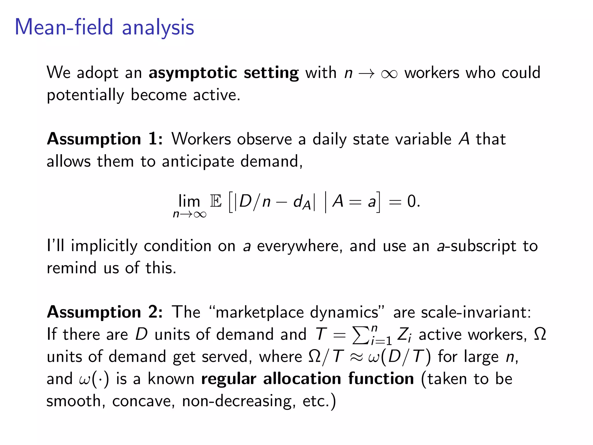
In order to correct for interference, we assume the following model:
The platform chooses a distribution π, and promises a
payment Pi
iid
∼ π to each worker.
If a fraction µ of workers are active, the expected amount of
demand served by any worker if they become active is q(µ).
Workers have random outside options Bi such that, given
the distribution π, the i-th worker is active with probability
fBi
(pi q(µ(π))) = 1/ (1 + exp [−β (pi q(µ(π)) − Bi )]) .
Note: the expected revenue of the i-th worker is pi q(µ(π)).
The system is in equilibrium, i.e., the fraction of active
workers is µ(π) = E [fBi
(pi q(µ(π)))].](https://image.slidesharecdn.com/wagner-expinequilibrium-191219170411/75/Causal-Inference-Opening-Workshop-Experimenting-in-Equilibrium-Stefan-Wager-December-9-2019-10-2048.jpg)
![A simple model
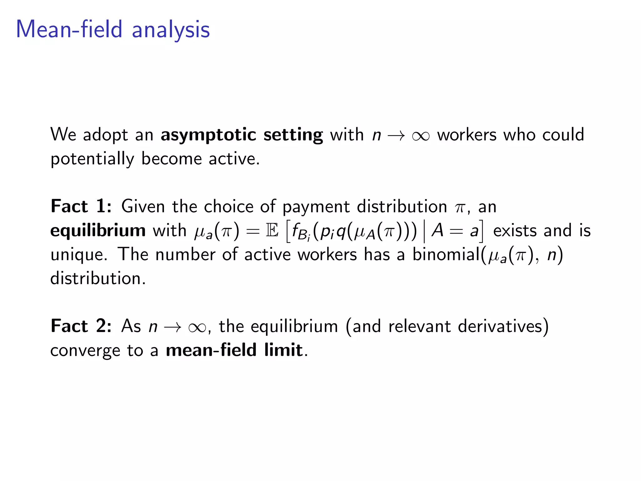
In order to correct for interference, we assume the following model:
The platform chooses a distribution π, and promises a
payment Pi
iid
∼ π to each worker.
If a fraction µ of workers are active and conditionally on daily
state A = a, the expected amount of demand served by
any worker if they become active is qa(µ).
Workers have random outside options Bi such that, given
the distribution π, the i-th worker is active with probability
fBi
(pi q(µ(π))) = 1/ (1 + exp [−β (pi q(µ(π)) − Bi )]) .
Note: the expected revenue of the i-th worker is pi q(µ(π)).
The system is in equilibrium, i.e., the fraction of active
workers is µa(π) = E fBi
(pi qA(µ(π))) A = a .
NB: The distribution of outside options Bi may depend on state A.](https://image.slidesharecdn.com/wagner-expinequilibrium-191219170411/75/Causal-Inference-Opening-Workshop-Experimenting-in-Equilibrium-Stefan-Wager-December-9-2019-17-2048.jpg)
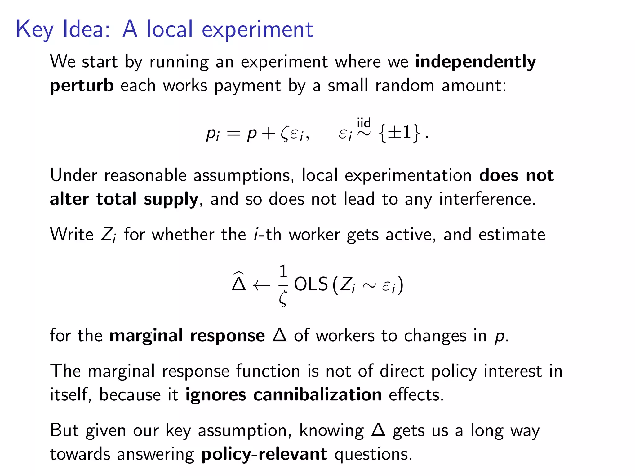
![Learning via Local Experimentation
The ultimate goal of the platform is to maximize its utility U, for
our purposes taken as total cost minus total revenue.
Write γ for the platform’s revenue per unit of demand served. In
the mean-field limit, the utility then converges to
n−1
Ua(p) = (γ − p) ω(da/µa(p)) µa(p), U(p) = E [UA(p)] .
Once we know dµa(p)/dp, working out the utility derivative
dUa(p)/dp amounts to calculus.
We consider a platform that uses these estimates to optimize U(p)
by gradient descent (or rather ascent).](https://image.slidesharecdn.com/wagner-expinequilibrium-191219170411/75/Causal-Inference-Opening-Workshop-Experimenting-in-Equilibrium-Stefan-Wager-December-9-2019-21-2048.jpg)
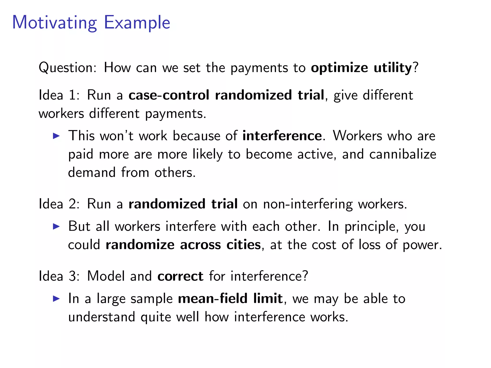
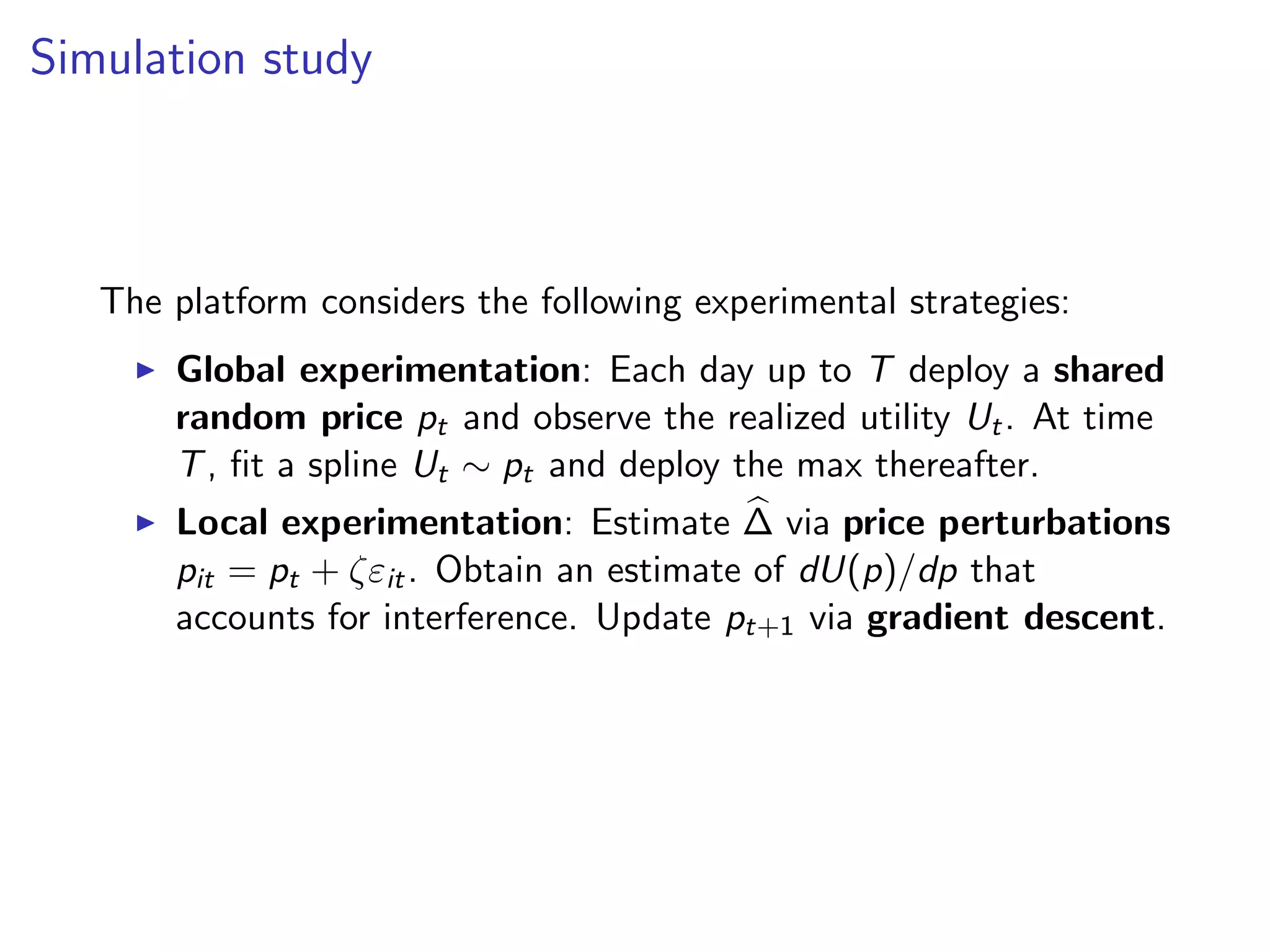
![A First-Order Algorithm
We now proceed to optimize payments via a variant of mirror
descent Specify a step size η, an interval I = [c−, c+], and an
initial payment p1. Then, at time period t = 1, 2, ...:
1. Deploy randomized payment perturbations εit around pt.
2. Estimate ∆ by regressing market participation on εit.
3. Translate this into an estimate Γt of dUAt (p)/dp via the
transformation implied by the mean-field limit.
4. Perform a gradient update, where θt = t
s=1 sΓs:
pt+1 = argminp
1
2η
t
s=1
s(p − ps)2
− θtp : p ∈ I
If the Ua(p) functions are strongly concave, this attains a 1/t rate
of convergence in large markets, both in regret and squared error.](https://image.slidesharecdn.com/wagner-expinequilibrium-191219170411/75/Causal-Inference-Opening-Workshop-Experimenting-in-Equilibrium-Stefan-Wager-December-9-2019-22-2048.jpg)
![A First-Order Algorithm
If the Ua(p) functions are strongly concave, this attains a 1/t rate
of convergence in large markets, both in regret and squared error.
Theorem. If the Ua(p) functions are σ-strongly concave,
|ua(p)| ≤ M, and we use a step size η > σ−1 then
lim
n→∞
P
1
T
T
t=1
t (UAt (p) − UAt (pt)) ≤
ηM2
2
= 1,
for any fixed payment p ∈ [c−, c+].
Corollary. If in addition the day-specific states At are IID, then
lim sup
n→∞
P (p∗
− ¯pT )2
≤
ηM2
σT
16 log δ−1
+ 4 ≥ 1 − δ,
p∗ = argmax {E [UA(p)] : p ∈ I} and ¯pT = 2
T(T+1)
T
t=1 t pt.](https://image.slidesharecdn.com/wagner-expinequilibrium-191219170411/75/Causal-Inference-Opening-Workshop-Experimenting-in-Equilibrium-Stefan-Wager-December-9-2019-23-2048.jpg)
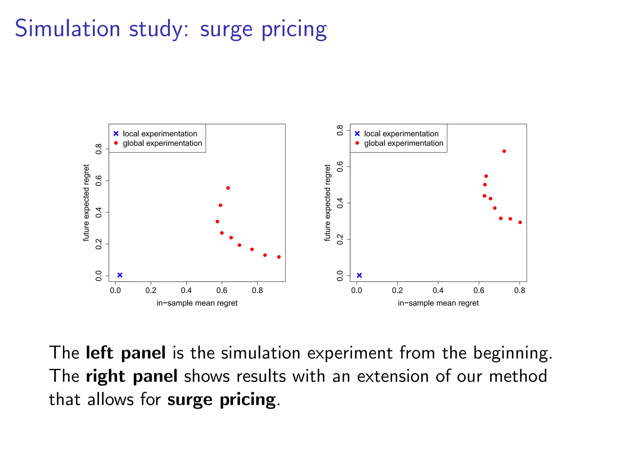


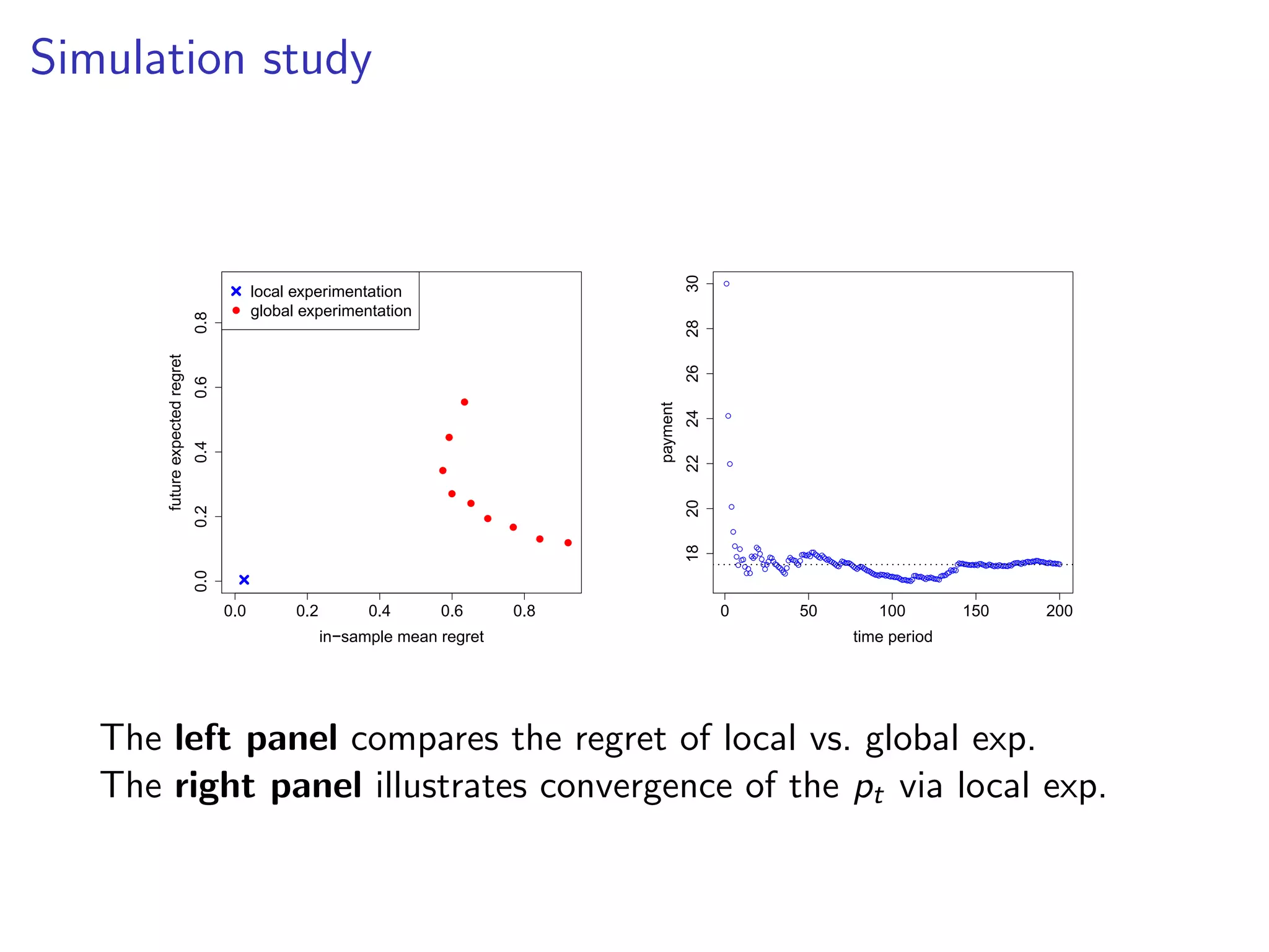
This document discusses challenges and strategies in optimizing payment structures for workers in sharing economy platforms through experimentation. It explores interference effects and proposes a local experimentation approach to efficiently estimate the marginal response of workers to payment changes while correcting for demand cannibalization. Simulation studies highlight the effectiveness of this method compared to traditional global experimentation in improving utility over time.