Download to read offline


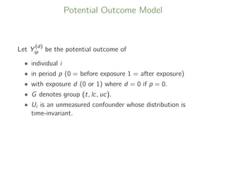
![Diff-in-Diff: Graphical Interpretation
-
6
r
r
r
r
t = 0 t = 1
E[R00]
E[R10]
E[R01]
E[R11|Z = 1]](https://image.slidesharecdn.com/keelesamsi2019-191219170607/85/Causal-Inference-Opening-Workshop-Bracketing-Bounds-for-Differences-in-Differences-Methods-Luke-Keele-December-10-2019-6-320.jpg)
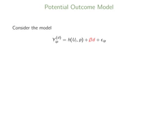
![Diff-in-Diff: Graphical Interpretation
-
6
r
r
r
r
t = 0 t = 1
E[R00]
E[R10]
E[R01]
E[R11|Z = 1]
b](https://image.slidesharecdn.com/keelesamsi2019-191219170607/85/Causal-Inference-Opening-Workshop-Bracketing-Bounds-for-Differences-in-Differences-Methods-Luke-Keele-December-10-2019-7-320.jpg)
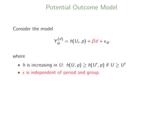
![Diff-in-Diff: Graphical Interpretation
-
6
r
r
r
r
t = 0 t = 1
E[R00]
E[R10]
E[R01]
E[R11|Z = 1]
bE[R11|Z = 0]](https://image.slidesharecdn.com/keelesamsi2019-191219170607/85/Causal-Inference-Opening-Workshop-Bracketing-Bounds-for-Differences-in-Differences-Methods-Luke-Keele-December-10-2019-8-320.jpg)
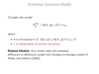
![Diff-in-Diff: Graphical Interpretation
-
6
r
r
r
r
t = 0 t = 1
E[R00]
E[R10]
E[R01]
E[R11|Z = 1]
bE[R11|Z = 0]
6
?
Treatment Effect](https://image.slidesharecdn.com/keelesamsi2019-191219170607/85/Causal-Inference-Opening-Workshop-Bracketing-Bounds-for-Differences-in-Differences-Methods-Luke-Keele-December-10-2019-9-320.jpg)


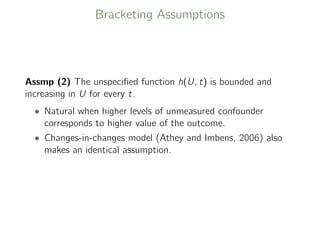
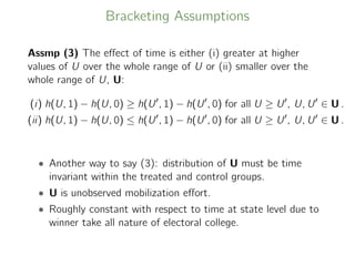
![Bracketing Assumptions
Assmp. (1) The within group distrbutions of U are stochastically
ordered:
U|G = lc U|G = t U|G = uc ,
meaning that
E[f (U)|G = lc] ≤ E[f (U)|G = t] ≤ E[f (U)|G = uc] for any
bounded, increasing function f .](https://image.slidesharecdn.com/keelesamsi2019-191219170607/85/Causal-Inference-Opening-Workshop-Bracketing-Bounds-for-Differences-in-Differences-Methods-Luke-Keele-December-10-2019-42-320.jpg)
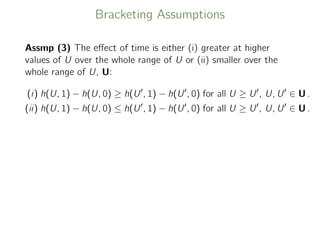
![Bracketing Assumptions
Assmp. (1) The within group distrbutions of U are stochastically
ordered:
U|G = lc U|G = t U|G = uc ,
meaning that
E[f (U)|G = lc] ≤ E[f (U)|G = t] ≤ E[f (U)|G = uc] for any
bounded, increasing function f .
• In words: Higher values of U correspond to higher outcomes.](https://image.slidesharecdn.com/keelesamsi2019-191219170607/85/Causal-Inference-Opening-Workshop-Bracketing-Bounds-for-Differences-in-Differences-Methods-Luke-Keele-December-10-2019-43-320.jpg)
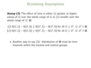
![Bracketing Assumptions
Assmp. (1) The within group distrbutions of U are stochastically
ordered:
U|G = lc U|G = t U|G = uc ,
meaning that
E[f (U)|G = lc] ≤ E[f (U)|G = t] ≤ E[f (U)|G = uc] for any
bounded, increasing function f .
• In words: Higher values of U correspond to higher outcomes.
• U is unobserved mobilization effort.](https://image.slidesharecdn.com/keelesamsi2019-191219170607/85/Causal-Inference-Opening-Workshop-Bracketing-Bounds-for-Differences-in-Differences-Methods-Luke-Keele-December-10-2019-44-320.jpg)
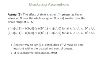
![Bracketing Assumptions
Assmp. (1) The within group distrbutions of U are stochastically
ordered:
U|G = lc U|G = t U|G = uc ,
meaning that
E[f (U)|G = lc] ≤ E[f (U)|G = t] ≤ E[f (U)|G = uc] for any
bounded, increasing function f .
• In words: Higher values of U correspond to higher outcomes.
• U is unobserved mobilization effort.
• Higher values of U likely lead to higher levels of turnout.](https://image.slidesharecdn.com/keelesamsi2019-191219170607/85/Causal-Inference-Opening-Workshop-Bracketing-Bounds-for-Differences-in-Differences-Methods-Luke-Keele-December-10-2019-45-320.jpg)
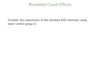
![Bracketed Causal Effects
Consider the expectation of the standard DiD estimator using
lower control group lc:
E ˆβdd.lc =
β + (E[h(U, 1) − h(U, 0)|G = t]) − (E[h(U, 1) − h(U, 0)|G = lc])](https://image.slidesharecdn.com/keelesamsi2019-191219170607/85/Causal-Inference-Opening-Workshop-Bracketing-Bounds-for-Differences-in-Differences-Methods-Luke-Keele-December-10-2019-52-320.jpg)
![Bracketed Causal Effects
Consider the expectation of the standard DiD estimator using
lower control group lc:
E ˆβdd.lc =
β + (E[h(U, 1) − h(U, 0)|G = t]) − (E[h(U, 1) − h(U, 0)|G = lc])
Similar logic yields,
E ˆβdd.uc =
β +(E[h(U, 1) − h(U, 0)|G = t])−(E[h(U, 1) − h(U, 0)|G = uc])](https://image.slidesharecdn.com/keelesamsi2019-191219170607/85/Causal-Inference-Opening-Workshop-Bracketing-Bounds-for-Differences-in-Differences-Methods-Luke-Keele-December-10-2019-53-320.jpg)
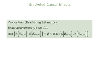


![DID Bracketing Estimates for Indiana
2008
DID Point Estimate 95% CI
Lower Control Group 4.4 [3.3, 5.4]
Upper Control Group 5.7 [4.2, 7.1]
Bounds [3.3, 7.1]
2012
DID Point Estimate 95% CI
Lower Control Group 5.9 [3.1, 8.6]
Upper Control Group 4.3 [3.3, 5.4]
Bounds [3.1, 8.6]](https://image.slidesharecdn.com/keelesamsi2019-191219170607/85/Causal-Inference-Opening-Workshop-Bracketing-Bounds-for-Differences-in-Differences-Methods-Luke-Keele-December-10-2019-63-320.jpg)
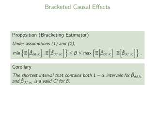
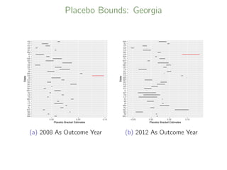
![DID Bracketing Estimates for Georgia
2008
DID Point Estimate 95% CI
Lower Control Group 9.8 [6.5, 13.1]
Upper Control Group 7.6 [6.3, 8.9]
Bounds [6.3, 13.1]
2012
DID Point Estimate 95% CI
Lower Control Group 13.4 [12.0, 14.8]
Upper Control Group 8.5 [6.7, 10.4]
Bounds [6.7, 14.8]](https://image.slidesharecdn.com/keelesamsi2019-191219170607/85/Causal-Inference-Opening-Workshop-Bracketing-Bounds-for-Differences-in-Differences-Methods-Luke-Keele-December-10-2019-64-320.jpg)
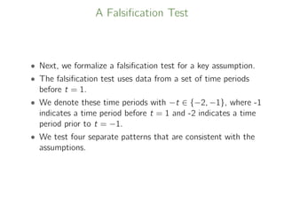
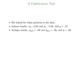
![A Falsification Test
The first pattern is
E[Y (−1)
|Zi = 1] − E[Y (−2)
|Zi = 1]
E[Y (−1)
|Zi = 0] − E[Y (−2)
|Zi = 0]
βuc,−t = E[Y (−1)
|Zi = 1] − E[Y (−2)
|Zi = 1] −
E[Y (−1)
|Zi = 0] − E[Y (−2)
|Zi = 0]
Test as: H(iii)[a] : βuc,−t 0 using p(iii)[a]](https://image.slidesharecdn.com/keelesamsi2019-191219170607/85/Causal-Inference-Opening-Workshop-Bracketing-Bounds-for-Differences-in-Differences-Methods-Luke-Keele-December-10-2019-77-320.jpg)
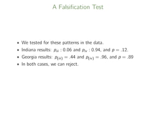
![A Falsification Test
The second pattern is
E[Y (−1)
|Di = 1] − E[Y (−2)
|Di = 1]
E[Y (−1)
|Di = 0] − E[Y (−2)
|Di = 0] .
Test as: H(iii)[b] : βlc,−t 0 using p(iii)[b]](https://image.slidesharecdn.com/keelesamsi2019-191219170607/85/Causal-Inference-Opening-Workshop-Bracketing-Bounds-for-Differences-in-Differences-Methods-Luke-Keele-December-10-2019-78-320.jpg)
![A Falsification Test
The third pattern is:
E[Y (−1)
|Zi = 1] − E[Y (−2)
|Zi = 1]
E[Y (−1)
|Zi = 0] − E[Y (−2)
|Zi = 0]
Test: H(iv)[a] : βuc,−t 0 using p(iv)[a]](https://image.slidesharecdn.com/keelesamsi2019-191219170607/85/Causal-Inference-Opening-Workshop-Bracketing-Bounds-for-Differences-in-Differences-Methods-Luke-Keele-December-10-2019-79-320.jpg)
![A Falsification Test
The fourth pattern is:
E[Y (−1)
|Di = 1] − E[Y (−2)
|Di = 1]
E[Y (−1)
|Di = 0] − E[Y (−2)
|Di = 0]
Test: H(iv)[a] : βul,−t 0 using p(iv)[b]](https://image.slidesharecdn.com/keelesamsi2019-191219170607/85/Causal-Inference-Opening-Workshop-Bracketing-Bounds-for-Differences-in-Differences-Methods-Luke-Keele-December-10-2019-80-320.jpg)
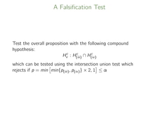
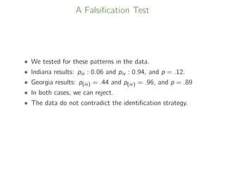
![A Falsification Test
Test Hc
(iii) with p(iii) = max{p(iii)[a], p(iii)[b]}
Test Hc
(iv) with p(iv) = max{p(iii)[a], p(iii)[b]}](https://image.slidesharecdn.com/keelesamsi2019-191219170607/85/Causal-Inference-Opening-Workshop-Bracketing-Bounds-for-Differences-in-Differences-Methods-Luke-Keele-December-10-2019-81-320.jpg)
![Sensitivity Analysis Bounds
The sensitivity bounds are:
LBsens = min[(τCIBBlb
−db2, τCIBBlb
−da), (τCIBBlb
−db, τCIBBlb
−da2)]
UBsens = max[(τCIBBub
− (−db2), τCIBBub
− (−da)),
(τCIBBub
− (−db), τCIBBub
− (−da2))]](https://image.slidesharecdn.com/keelesamsi2019-191219170607/85/Causal-Inference-Opening-Workshop-Bracketing-Bounds-for-Differences-in-Differences-Methods-Luke-Keele-December-10-2019-93-320.jpg)
![Sensitivity Analysis
Table: Sensitivity Analysis for Indiana
2008
DID Bracketing Bounds [3.3, 7.1]
Sensitivity Analysis Bounds [1.7, 12.0]
2012
DID Bracketing Bounds [3.1, 8.6]
Sensitivity Analysis Bounds [0.0, 18.0]](https://image.slidesharecdn.com/keelesamsi2019-191219170607/85/Causal-Inference-Opening-Workshop-Bracketing-Bounds-for-Differences-in-Differences-Methods-Luke-Keele-December-10-2019-94-320.jpg)
![Sensitivity Analysis
Table: Sensitivity Analysis for Georgia
2008
DID Bracketing Bounds [6.3, 13.1]
Sensitivity Analysis Bounds [1.2, 13.6]
2012
DID Bracketing Bounds [6.7, 14.8]
Sensitivity Analysis Bounds [-1.2, 15.0]](https://image.slidesharecdn.com/keelesamsi2019-191219170607/85/Causal-Inference-Opening-Workshop-Bracketing-Bounds-for-Differences-in-Differences-Methods-Luke-Keele-December-10-2019-95-320.jpg)
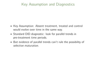
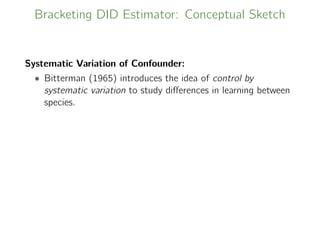
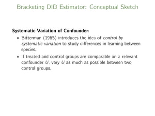
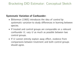
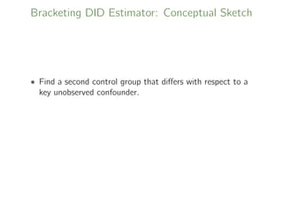
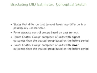
The document discusses the use of differences-in-differences (DiD) methodology for estimating causal effects, specifically in the context of voter ID laws in Indiana and Georgia. It reviews assumptions, diagnostics, and introduces a new bracketing estimator to address potential confounding effects arising from selective maturation. Key findings highlight the importance of constructing appropriate control groups based on past turnout levels to improve the accuracy of causal estimates in electoral studies.