Download to read offline
![EnKF with super-meshing (1D-case)
Guider et al., 2017 (In preparation)
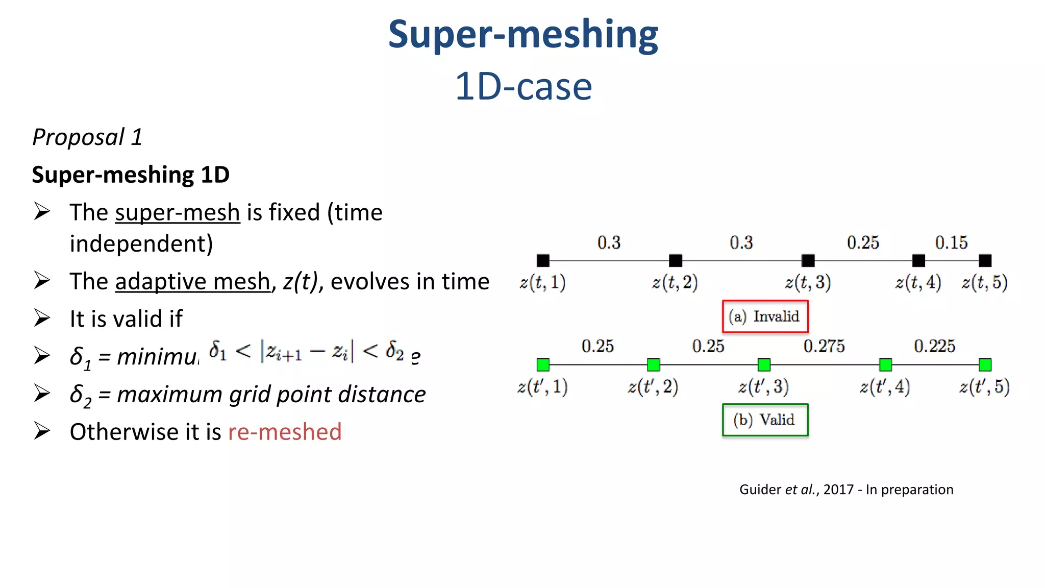
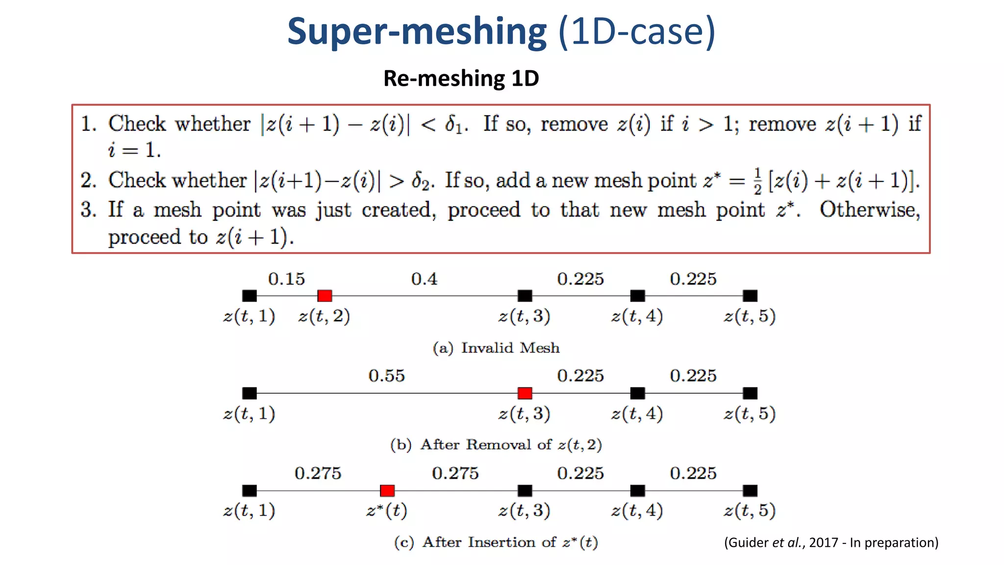
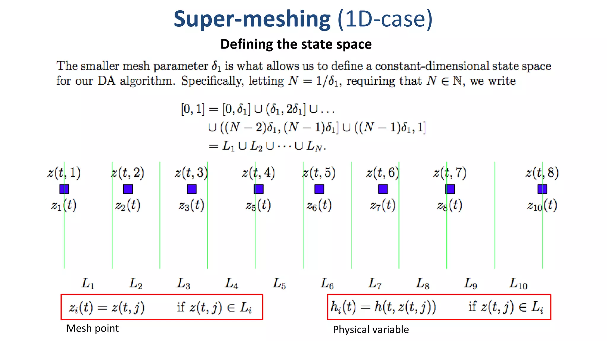
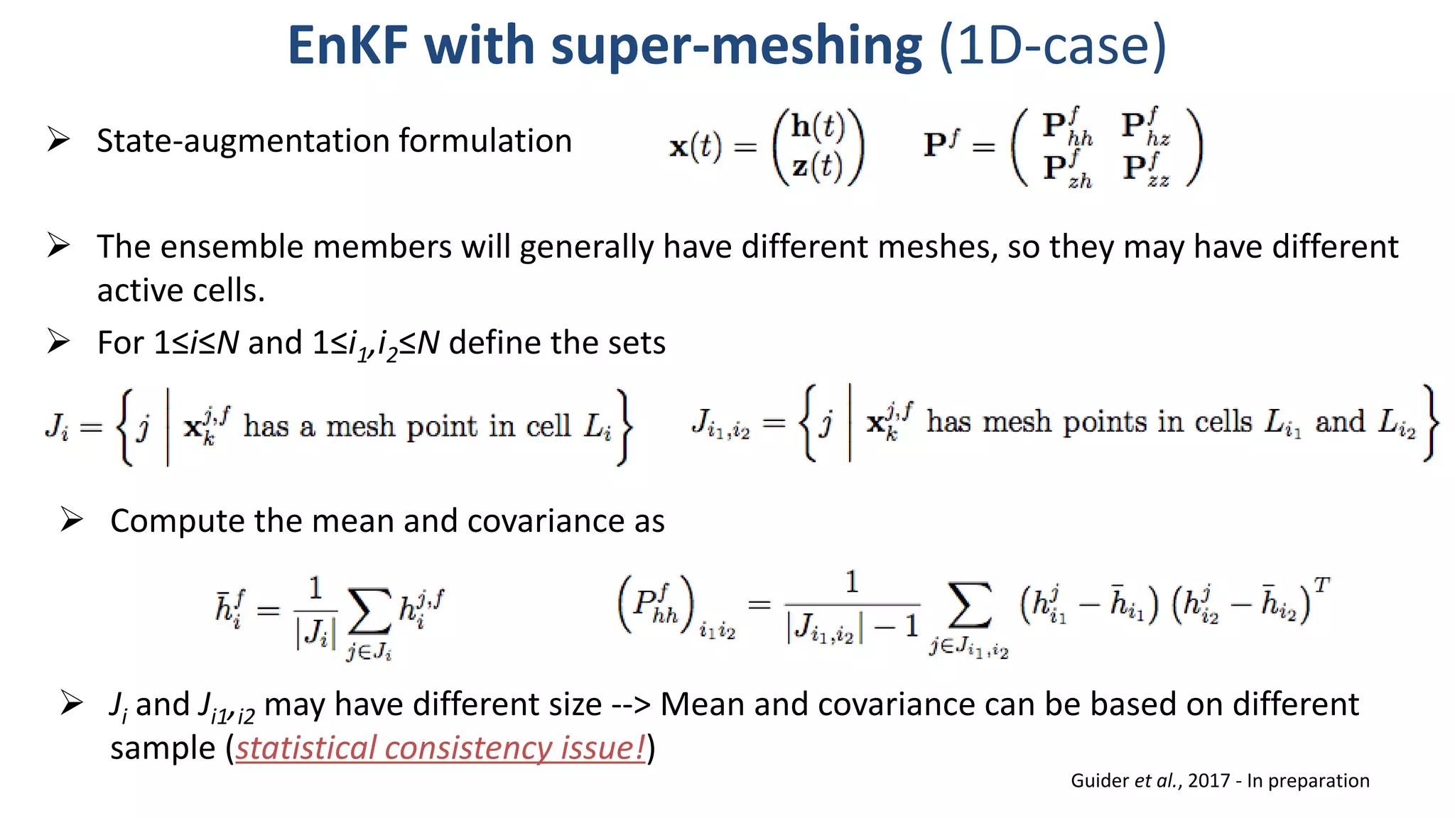
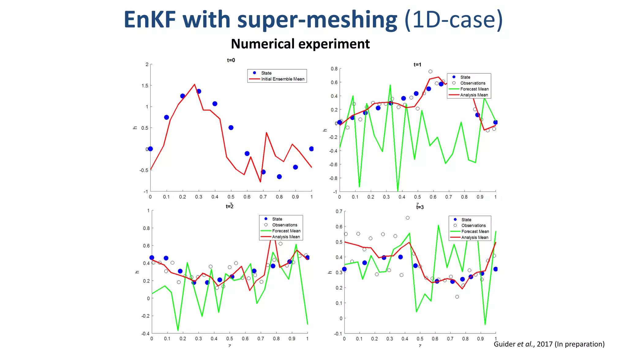
Numerical experiment
The adaptive mesh, z(t), evolves as
The physical variable, h(t), evolves
following the Burgers’ equation
The fixed super-mesh has N=50 cells and δ1/δ2 =
0.05/0.15
EnKF with Ne=50 members
25 observations evenly spaced over [0,1]](https://image.slidesharecdn.com/carrassidataassimilation-170828221436/75/Program-on-Mathematical-and-Statistical-Methods-for-Climate-and-the-Earth-System-Opening-Workshop-Issues-in-Ensemble-Prediction-and-Data-Assimilation-Using-a-Lagrangian-Model-of-Sea-Ice-Alberto-Carrassi-Aug-22-2017-26-2048.jpg)
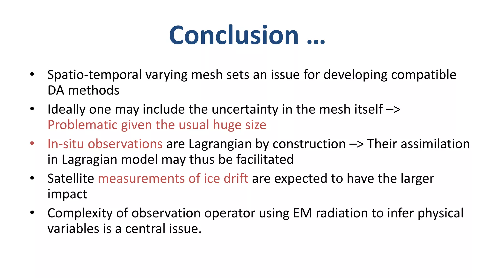
The document presents a new Lagrangian model for sea ice that addresses the shortcomings of existing methods, particularly in data assimilation and ice mechanics. It discusses the operational and simulation performance of the model, including comparisons with previous systems, and highlights issues like biases, variability, and the need for better data assimilation techniques. The findings emphasize the model's capability to simulate sea ice dynamics accurately, while proposing new methodologies for integrated data approaches.