Download as PDF, PPTX


![Open Questions
28
• What are appropriate coarse-grained parcelations of a brain?
- How can we discover them?
• How do we handle time delays?
- (sampling rate)
- slower vs. faster causal effects
• How to model the interventions?
- (soft vs. hard)
- time course of the intervention
- electric stimulation vs. task fMRI vs. magnetic stimulation
• What is the relation between the observational network and
the stimulated network?
• [scalability of methods with weaker assumptions: fast non-
parametric independence tests; non-Gaussian / non-linear
methods etc.]](https://image.slidesharecdn.com/causaldiscneuroimagingfeberhardt-191231210935/75/Causal-Inference-Opening-Workshop-Causal-Discovery-in-Neuroimaging-Data-Frederick-Eberhardt-December-11-2019-66-2048.jpg)

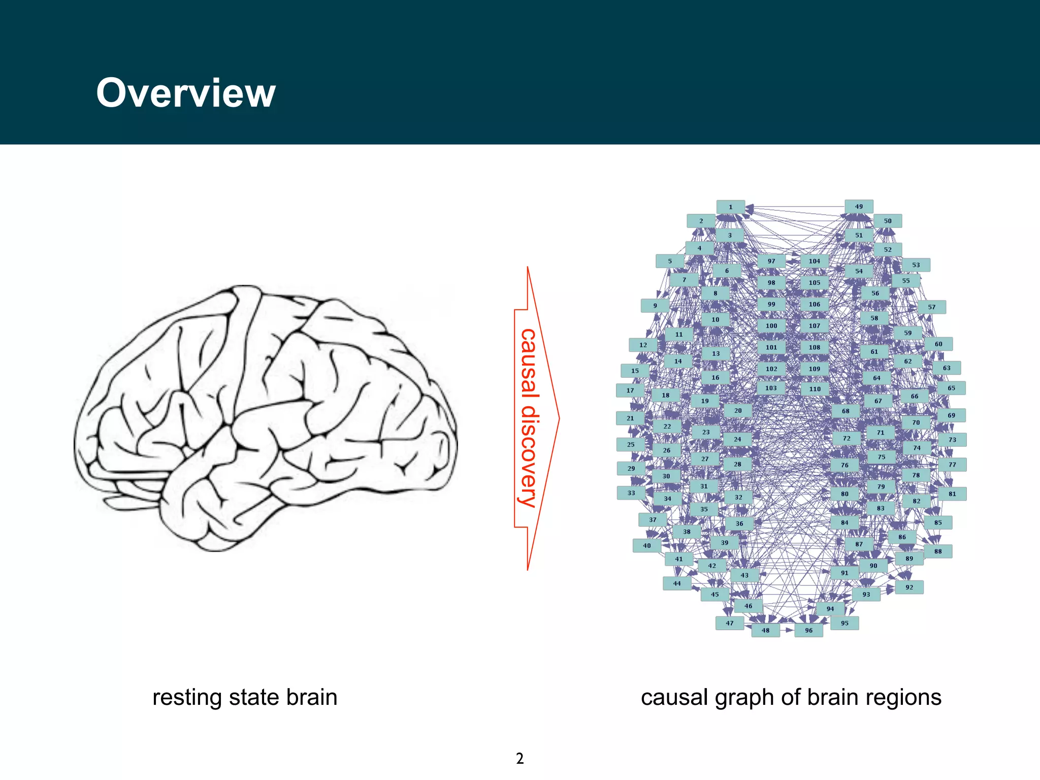
The document discusses causal discovery in neuroimaging data, specifically focusing on resting state fMRI from the Human Connectome Project. It outlines the experimental setup, including parameters for data acquisition and the nature of measurements taken, such as the correlation of bold signals across multiple brain regions. The aim is to analyze interactions and neural activity across a vast number of neurons and voxels over time.