Download as PDF, PPTX


![INPUT
[DATA]
PREDICTION
Machine
Learning](https://image.slidesharecdn.com/zlabeieee-grss12-07-2022-221204192030-876ba38c/85/Machine-learning-for-evaluating-climate-model-projections-18-320.jpg)
![INPUT
[DATA]
PREDICTION
~Statistical
Algorithm~](https://image.slidesharecdn.com/zlabeieee-grss12-07-2022-221204192030-876ba38c/85/Machine-learning-for-evaluating-climate-model-projections-19-320.jpg)
![INPUT
[DATA]
PREDICTION
Machine
Learning](https://image.slidesharecdn.com/zlabeieee-grss12-07-2022-221204192030-876ba38c/85/Machine-learning-for-evaluating-climate-model-projections-20-320.jpg)


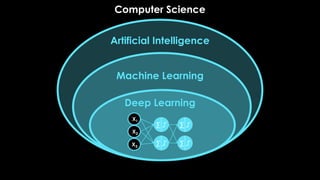
![X1
X2
INPUTS
Artificial Neural Networks [ANN]](https://image.slidesharecdn.com/zlabeieee-grss12-07-2022-221204192030-876ba38c/85/Machine-learning-for-evaluating-climate-model-projections-25-320.jpg)
![Linear regression!
Artificial Neural Networks [ANN]
X1
X2
W1
W2
∑ = X1W1+ X2W2 + b
INPUTS
NODE](https://image.slidesharecdn.com/zlabeieee-grss12-07-2022-221204192030-876ba38c/85/Machine-learning-for-evaluating-climate-model-projections-26-320.jpg)
![Artificial Neural Networks [ANN]
X1
X2
W1
W2
∑
INPUTS
NODE
Linear regression with non-linear
mapping by an “activation function”
Training of the network is merely
determining the weights “w” and
bias/offset “b"
= factivation(X1W1+ X2W2 + b)](https://image.slidesharecdn.com/zlabeieee-grss12-07-2022-221204192030-876ba38c/85/Machine-learning-for-evaluating-climate-model-projections-27-320.jpg)
![Artificial Neural Networks [ANN]
X1
X2
W1
W2
∑
INPUTS
NODE
= factivation(X1W1+ X2W2 + b)
ReLU Sigmoid Linear](https://image.slidesharecdn.com/zlabeieee-grss12-07-2022-221204192030-876ba38c/85/Machine-learning-for-evaluating-climate-model-projections-28-320.jpg)
![X1
X2
∑
inputs
HIDDEN LAYERS
X3
∑
∑
∑
OUTPUT
= predictions
Artificial Neural Networks [ANN]
: : ::
INPUTS](https://image.slidesharecdn.com/zlabeieee-grss12-07-2022-221204192030-876ba38c/85/Machine-learning-for-evaluating-climate-model-projections-29-320.jpg)
![Complexity and nonlinearities of the ANN allow it to learn many
different pathways of predictable behavior
Once trained, you have an array of weights and biases which can be
used for prediction on new data
INPUT
[DATA]
PREDICTION
Artificial Neural Networks [ANN]](https://image.slidesharecdn.com/zlabeieee-grss12-07-2022-221204192030-876ba38c/85/Machine-learning-for-evaluating-climate-model-projections-30-320.jpg)

![----ANN----
2 Hidden Layers
10 Nodes each
Ridge Regularization
Early Stopping
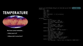
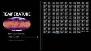
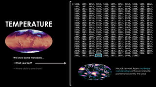
We know some metadata…
+ What year is it?
+ Where did it come from?
[e.g., Barnes et al. 2019, 2020]
[e.g., Labe and Barnes, 2021]
TIMING OF EMERGENCE
(COMBINED VARIABLES)
RESPONSES TO
EXTERNAL CLIMATE
FORCINGS
PATTERNS OF
CLIMATE INDICATORS
[e.g., Rader et al. 2022]
Surface Temperature Map Precipitation Map
+
TEMPERATURE](https://image.slidesharecdn.com/zlabeieee-grss12-07-2022-221204192030-876ba38c/85/Machine-learning-for-evaluating-climate-model-projections-35-320.jpg)
![----ANN----
2 Hidden Layers
10 Nodes each
Ridge Regularization
Early Stopping
We know some metadata…
+ What year is it?
+ Where did it come from?
[e.g., Barnes et al. 2019, 2020]
[e.g., Labe and Barnes, 2021]
TIMING OF EMERGENCE
(COMBINED VARIABLES)
RESPONSES TO
EXTERNAL CLIMATE
FORCINGS
PATTERNS OF
CLIMATE INDICATORS
Surface Temperature Map Precipitation Map
+
TEMPERATURE
[e.g., Rader et al. 2022]](https://image.slidesharecdn.com/zlabeieee-grss12-07-2022-221204192030-876ba38c/85/Machine-learning-for-evaluating-climate-model-projections-36-320.jpg)
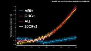
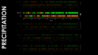
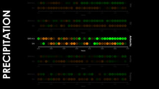
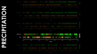
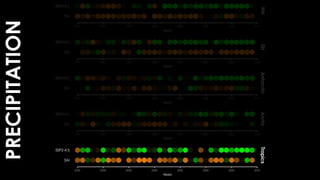
![Greenhouse gases fixed to 1920 levels
All forcings (CESM-LE)
Industrial aerosols fixed to 1920 levels
[Deser et al. 2020, JCLI]
Fully-coupled CESM1.1
20 Ensemble Members
Run from 1920-2080
Observations](https://image.slidesharecdn.com/zlabeieee-grss12-07-2022-221204192030-876ba38c/85/Machine-learning-for-evaluating-climate-model-projections-49-320.jpg)

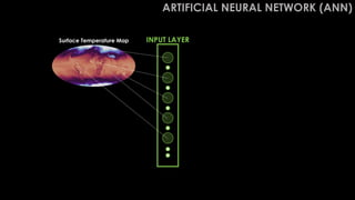
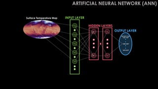
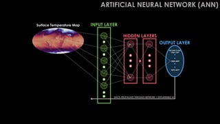
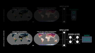
![INPUT LAYER
HIDDEN LAYERS
OUTPUT LAYER
Layer-wise Relevance Propagation
Surface Temperature Map
“2000-2009”
DECADE CLASS
“2070-2079”
“1920-1929”
BACK-PROPAGATE THROUGH NETWORK = EXPLAINABLE AI
ARTIFICIAL NEURAL NETWORK (ANN)
[Barnes et al. 2020, JAMES]
[Labe and Barnes 2021, JAMES]](https://image.slidesharecdn.com/zlabeieee-grss12-07-2022-221204192030-876ba38c/85/Machine-learning-for-evaluating-climate-model-projections-55-320.jpg)
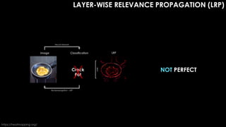
![[Adapted from Adebayo et al., 2020]
EXPLAINABLE AI IS
NOT PERFECT
THERE ARE MANY
METHODS](https://image.slidesharecdn.com/zlabeieee-grss12-07-2022-221204192030-876ba38c/85/Machine-learning-for-evaluating-climate-model-projections-60-320.jpg)
![[Adapted from Adebayo et al., 2020]
THERE ARE MANY
METHODS
EXPLAINABLE AI IS
NOT PERFECT](https://image.slidesharecdn.com/zlabeieee-grss12-07-2022-221204192030-876ba38c/85/Machine-learning-for-evaluating-climate-model-projections-61-320.jpg)
![OUTPUT LAYER
Layer-wise Relevance Propagation
“2000-2009”
DECADE CLASS
“2070-2079”
“1920-1929”
BACK-PROPAGATE THROUGH NETWORK = EXPLAINABLE AI
WHY?
= LRP HEAT MAPS
[Labe and Barnes 2021, JAMES]](https://image.slidesharecdn.com/zlabeieee-grss12-07-2022-221204192030-876ba38c/85/Machine-learning-for-evaluating-climate-model-projections-62-320.jpg)
![Layer-wise Relevance Propagation
BACK-PROPAGATE THROUGH NETWORK = EXPLAINABLE AI
WHY?
= LRP HEAT MAPS
Machine Learning
Black Box
[Labe and Barnes 2021, JAMES]](https://image.slidesharecdn.com/zlabeieee-grss12-07-2022-221204192030-876ba38c/85/Machine-learning-for-evaluating-climate-model-projections-63-320.jpg)
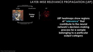
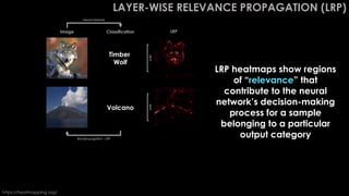
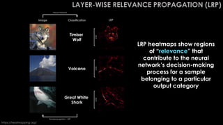
![Layer-wise Relevance Propagation
BACK-PROPAGATE THROUGH NETWORK = EXPLAINABLE AI
WHY?
= LRP HEAT MAPS
Find regions of “relevance”
that contribute to the
neural network’s
decision-making process
[Labe and Barnes 2021, JAMES]](https://image.slidesharecdn.com/zlabeieee-grss12-07-2022-221204192030-876ba38c/85/Machine-learning-for-evaluating-climate-model-projections-64-320.jpg)
![1960-1999: ANNUAL MEAN TEMPERATURE TRENDS
Greenhouse gases fixed
to 1920 levels
[AEROSOLS PREVAIL]
Industrial aerosols fixed
to 1920 levels
[GREENHOUSE GASES PREVAIL]
All forcings
[STANDARD CESM-LE]
DATA](https://image.slidesharecdn.com/zlabeieee-grss12-07-2022-221204192030-876ba38c/85/Machine-learning-for-evaluating-climate-model-projections-65-320.jpg)
![1960-1999: ANNUAL MEAN TEMPERATURE TRENDS
Greenhouse gases fixed
to 1920 levels
[AEROSOLS PREVAIL]
Industrial aerosols fixed
to 1920 levels
[GREENHOUSE GASES PREVAIL]
All forcings
[STANDARD CESM-LE]
DATA](https://image.slidesharecdn.com/zlabeieee-grss12-07-2022-221204192030-876ba38c/85/Machine-learning-for-evaluating-climate-model-projections-66-320.jpg)
![1960-1999: ANNUAL MEAN TEMPERATURE TRENDS
Greenhouse gases fixed
to 1920 levels
[AEROSOLS PREVAIL]
Industrial aerosols fixed
to 1920 levels
[GREENHOUSE GASES PREVAIL]
All forcings
[STANDARD CESM-LE]
DATA](https://image.slidesharecdn.com/zlabeieee-grss12-07-2022-221204192030-876ba38c/85/Machine-learning-for-evaluating-climate-model-projections-67-320.jpg)
![1960-1999: ANNUAL MEAN TEMPERATURE TRENDS
Greenhouse gases fixed
to 1920 levels
[AEROSOLS PREVAIL]
Industrial aerosols fixed
to 1920 levels
[GREENHOUSE GASES PREVAIL]
All forcings
[STANDARD CESM-LE]
DATA](https://image.slidesharecdn.com/zlabeieee-grss12-07-2022-221204192030-876ba38c/85/Machine-learning-for-evaluating-climate-model-projections-68-320.jpg)
![CLIMATE MODEL DATA PREDICT THE YEAR FROM MAPS OF TEMPERATURE
AEROSOLS
PREVAIL
GREENHOUSE GASES
PREVAIL
STANDARD
CLIMATE MODEL
[Labe and Barnes 2021, JAMES]](https://image.slidesharecdn.com/zlabeieee-grss12-07-2022-221204192030-876ba38c/85/Machine-learning-for-evaluating-climate-model-projections-69-320.jpg)
![OBSERVATIONS PREDICT THE YEAR FROM MAPS OF TEMPERATURE
AEROSOLS
PREVAIL
GREENHOUSE GASES
PREVAIL
STANDARD
CLIMATE MODEL
[Labe and Barnes 2021, JAMES]](https://image.slidesharecdn.com/zlabeieee-grss12-07-2022-221204192030-876ba38c/85/Machine-learning-for-evaluating-climate-model-projections-70-320.jpg)
![OBSERVATIONS
SLOPES
PREDICT THE YEAR FROM MAPS OF TEMPERATURE
AEROSOLS
PREVAIL
GREENHOUSE GASES
PREVAIL
STANDARD
CLIMATE MODEL
[Labe and Barnes 2021, JAMES]](https://image.slidesharecdn.com/zlabeieee-grss12-07-2022-221204192030-876ba38c/85/Machine-learning-for-evaluating-climate-model-projections-71-320.jpg)
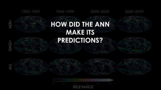
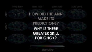
![RESULTS FROM LRP
[Labe and Barnes 2021, JAMES]
Low High](https://image.slidesharecdn.com/zlabeieee-grss12-07-2022-221204192030-876ba38c/85/Machine-learning-for-evaluating-climate-model-projections-74-320.jpg)
![RESULTS FROM LRP
[Labe and Barnes 2021, JAMES]
Low High](https://image.slidesharecdn.com/zlabeieee-grss12-07-2022-221204192030-876ba38c/85/Machine-learning-for-evaluating-climate-model-projections-75-320.jpg)
![RESULTS FROM LRP
[Labe and Barnes 2021, JAMES]
Low High](https://image.slidesharecdn.com/zlabeieee-grss12-07-2022-221204192030-876ba38c/85/Machine-learning-for-evaluating-climate-model-projections-76-320.jpg)
![RESULTS FROM LRP
[Labe and Barnes 2021, JAMES]
Low High](https://image.slidesharecdn.com/zlabeieee-grss12-07-2022-221204192030-876ba38c/85/Machine-learning-for-evaluating-climate-model-projections-77-320.jpg)


![INPUT
[DATA]
PREDICTION
Machine
Learning
Explainable AI
Learn new
science!](https://image.slidesharecdn.com/zlabeieee-grss12-07-2022-221204192030-876ba38c/85/Machine-learning-for-evaluating-climate-model-projections-113-320.jpg)


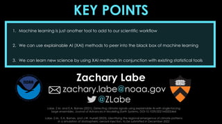

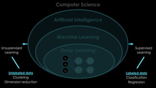
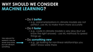
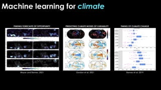
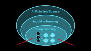
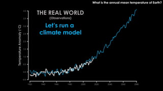
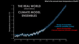
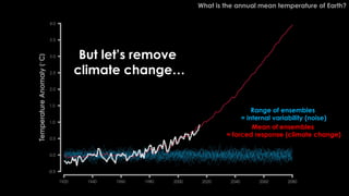
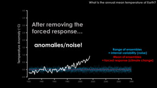
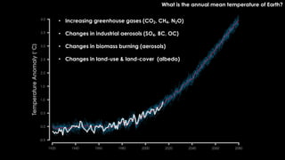
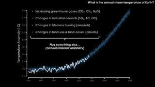
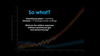
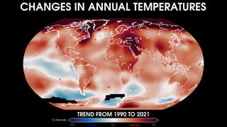
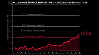
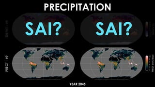
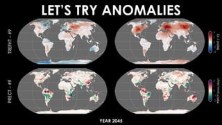
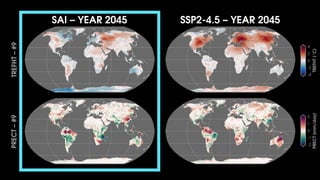
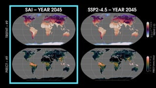
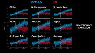
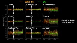
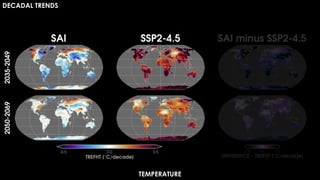
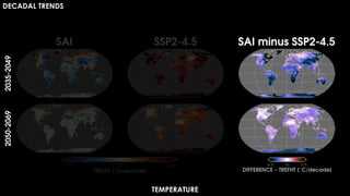
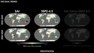
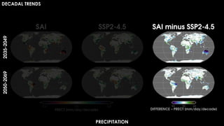
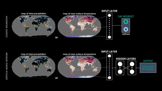
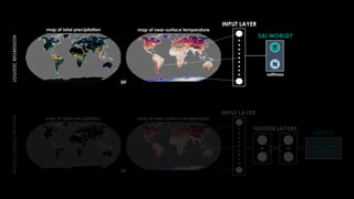
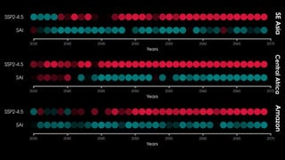
The document discusses the application of machine learning (ML) in evaluating climate model projections, highlighting its potential to enhance accuracy, speed, and uncover new relationships within climate data. It describes various ML techniques, specifically artificial neural networks, and their roles in predicting climate phenomena and improving weather forecasts. Key takeaways include the integration of explainable AI to deepen understanding of ML predictions, allowing researchers to gain insights into climate data and models.


![谷歌留痕技术 [ 𝙩𝙤𝙥 𝟮𝟯𝟯. 𝙘 𝙤𝙢 ]](https://cdn.slidesharecdn.com/ss_thumbnails/top233-260130174328-3833018c-thumbnail.jpg?width=640&height=640&fit=bounds)


