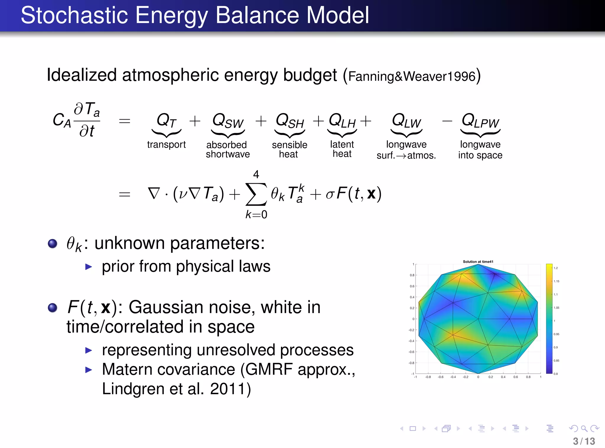
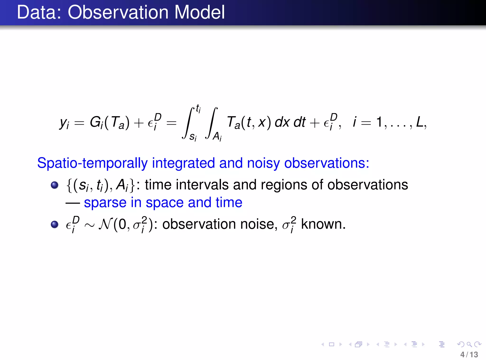
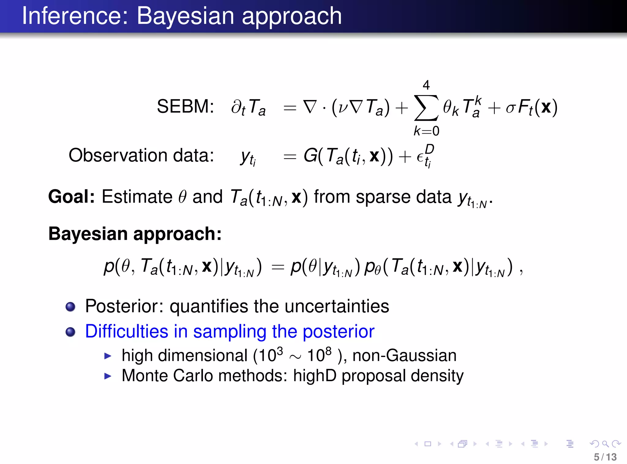
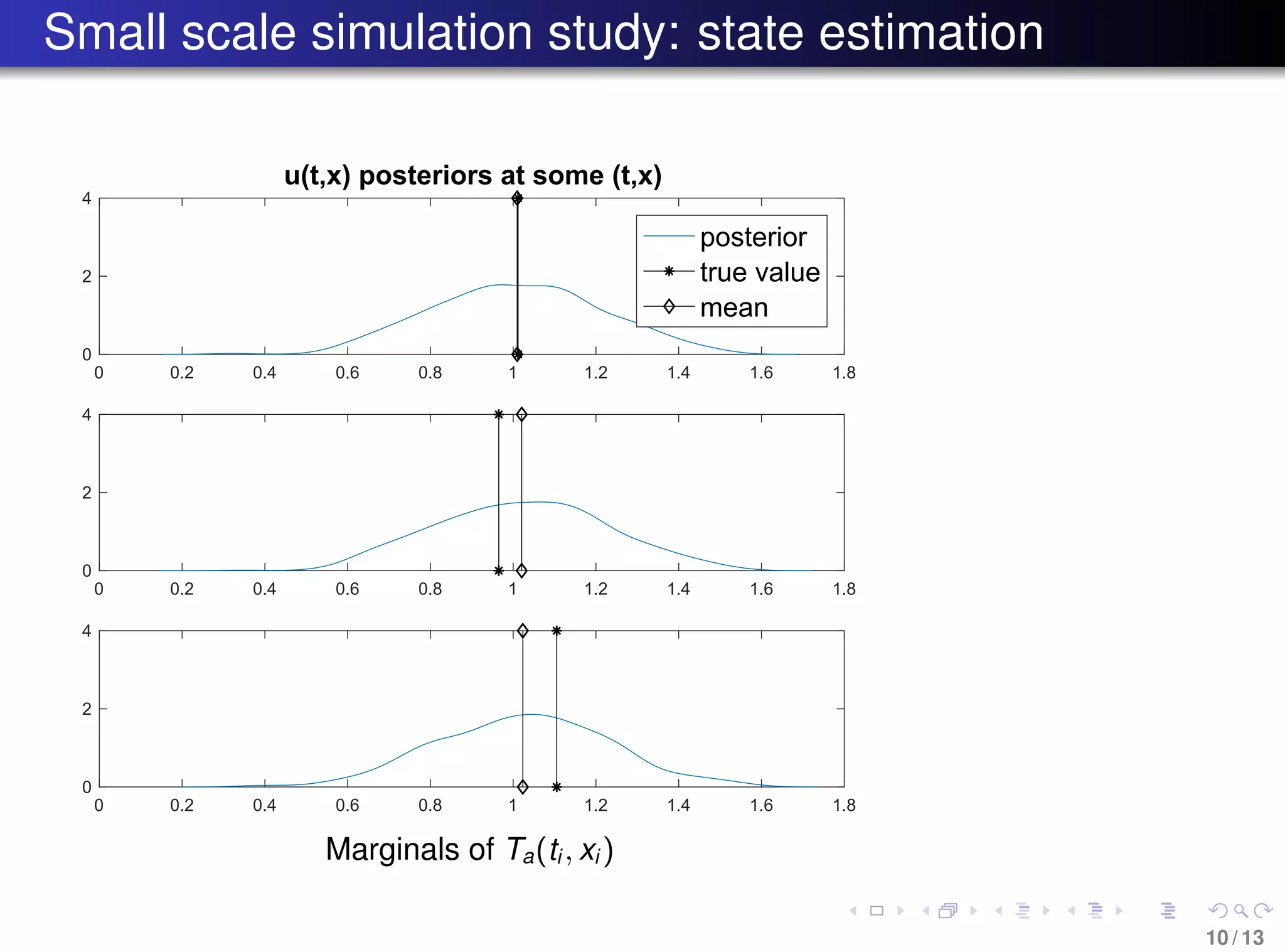
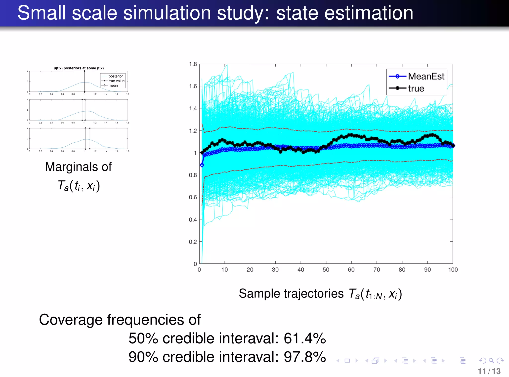
The document discusses the reconstruction of historical temperature variations during the last deglaciation using a Bayesian approach and a stochastic energy balance model. It focuses on estimating parameters and states from sparse, noisy observational data and employs Particle MCMC for efficient sampling in high-dimensional space. The findings indicate a method to analyze climate response to external changes and improve climate modeling techniques.

1. Bayesian Climate Reconstructions
using Stochastic Energy Balance Models
Fei Lu 1 Nils Weitzel2 Adam Monahan3
1Department of Mathematics, Johns Hopkins
2Meteorological Institute, University of Bonn, Germany
3School of Earth and Ocean Science, University of Victoria, Canada
SAMSI Climate Transition Workshop
May 15, 2018
1 / 13

2. Motivation
Goal: Reconstruction of spatio-temporal evolution of temperature
during the last deglaciation (from ∼21ky BP to ∼ 6ky BP)
important for understanding of gradual and abrupt climate changes
allows testing of climate models under different forcing conditions
find long-term constraints on climate response to changes in external forcings
Data: Indirect measurements (expensive) → sparse noisy data
Bayesian approach:
physically motivated stochastic energy balance model
proxy data
infer physically reasonable, data constraint model and fields
2 / 13

3. Stochastic Energy Balance Model
Idealized atmospheric energy budget (Fanning&Weaver1996)
CA
∂Ta
∂t
= QT
transport
+ QSW
absorbed
shortwave
+ QSH
sensible
heat
+ QLH
latent
heat
+ QLW
longwave
surf.→atmos.
− QLPW
longwave
into space
= · (ν Ta) +
4
k=0
θk Tk
a + σF(t, x)
θk : unknown parameters:
prior from physical laws
F(t, x): Gaussian noise, white in
time/correlated in space
representing unresolved processes
Matern covariance (GMRF approx.,
Lindgren et al. 2011)
3 / 13

4. Data: Observation Model
yi = Gi(Ta) + D
i =
ti
si Ai
Ta(t, x) dx dt + D
i , i = 1, . . . , L,
Spatio-temporally integrated and noisy observations:
{(si, ti), Ai}: time intervals and regions of observations
— sparse in space and time
D
i ∼ N(0, σ2
i ): observation noise, σ2
i known.
4 / 13

5. Inference: Bayesian approach
SEBM: ∂t Ta = · (ν Ta) +
4
k=0
θk Tk
a + σFt (x)
Observation data: yti
= G(Ta(ti, x)) + D
ti
Goal: Estimate θ and Ta(t1:N, x) from sparse data yt1:N
.
Bayesian approach:
p(θ, Ta(t1:N, x)|yt1:N
) = p(θ|yt1:N
) pθ(Ta(t1:N, x)|yt1:N
) ,
Posterior: quantifies the uncertainties
Difficulties in sampling the posterior
high dimensional (103
∼ 108
), non-Gaussian
Monte Carlo methods: highD proposal density
5 / 13

6. Sampling: particle MCMC
Particle MCMC (Andrieu&Doucet&Holenstein10)
Combines Sequential MC with MCMC:
SMC: seq. importance sampling → highD proposal density
MCMC transition by conditional SMC
→ target distr invariant (global feature) even w/ 5 particles
⇒ Efficient sampling of highD and highly correlated state
trajectory of state-space model.
Particle Gibbs with Ancestor Sampling (Lindsten&Jordan&Schon14)
sample the ancestor index using the weights
efficient forward step → fast mixing through conditional SMC.
6 / 13

7. Small scale simulation study:
Physical settings:
prior of the parameters: uniform
θ0 θ1 θ2 θ3 θ4
lower bound 0.8 -0.2 0 -0.2 -1.2
upper bound 1.2 0 0.4 0 -0.8
temperature near an equilibrium
point (normalized to be 1)
Scale in test: 4 × 103
42 spatial nodes
100 time steps
observe 40 regions (3 elements
each) each time;
Discretization:
FD in time
FEM in space
7 / 13

8. Small scale simulation study: parameter estimation
-2 -1 0 1 2 3 4 5 6 7
0
1
2
Theta posteriors
posterior
true value
mean
-2 -1.5 -1 -0.5 0 0.5 1 1.5 2 2.5
0
2
4
-0.5 0 0.5 1 1.5 2 2.5 3
0
2
4
-3 -2 -1 0 1 2 3 4 5
0
2
4
-2 -1 0 1 2 3 4 5 6
0
1
2
Marginals of the posterior
8 / 13

9. Small scale simulation study: parameter estimation
-2 -1 0 1 2 3 4 5 6 7
0
1
2
Theta posteriors
posterior
true value
mean
-2 -1.5 -1 -0.5 0 0.5 1 1.5 2 2.5
0
2
4
-0.5 0 0.5 1 1.5 2 2.5 3
0
2
4
-3 -2 -1 0 1 2 3 4 5
0
2
4
-2 -1 0 1 2 3 4 5 6
0
1
2
Marginals of the posterior
Scatter plots
9 / 13

10. Small scale simulation study: state estimation
0 0.2 0.4 0.6 0.8 1 1.2 1.4 1.6 1.8
0
2
4
u(t,x) posteriors at some (t,x)
posterior
true value
mean
0 0.2 0.4 0.6 0.8 1 1.2 1.4 1.6 1.8
0
2
4
0 0.2 0.4 0.6 0.8 1 1.2 1.4 1.6 1.8
0
2
4
Marginals of Ta(ti , xi )
10 / 13

11. Small scale simulation study: state estimation
0 0.2 0.4 0.6 0.8 1 1.2 1.4 1.6 1.8
0
2
4
u(t,x) posteriors at some (t,x)
posterior
true value
mean
0 0.2 0.4 0.6 0.8 1 1.2 1.4 1.6 1.8
0
2
4
0 0.2 0.4 0.6 0.8 1 1.2 1.4 1.6 1.8
0
2
4
Marginals of
Ta(ti , xi )
Sample trajectories Ta(t1:N , xi )
Coverage frequencies of
50% credible interaval: 61.4%
90% credible interaval: 97.8%
11 / 13

12. Summary and outlook
Bayesian construction of spatial-temporal temperature
a stochastic energy balance model
physically motivated SPDE
FEM on sphere, backward Euler in time,
sparse and noisy data
Estimate both parameters and states
Sample the posterior by particle MCMC
12 / 13

13. Summary and outlook
Bayesian construction of spatial-temporal temperature
Outlook:
Algorithm aspects:
criteria of performance (samples of the random field)
algorithm scale-up (more grid points/time steps)
parallel the SMC particles
MCMC stop creteria
Climatological issues:
Determine relevant fields for forcing terms (with reasonable priors
for parameters)
Pseudo-proxy experiments with simulation for deglaciation
(CCSM3 TraCE21K, Liu et al. 2009)
Apply to state-of-the-art proxy synthesis
13 / 13