Downloaded 11 times
![Data fusion: an old problem
• Often, observations of the inital states are not available: this
was recognized by mathematicians and astronomers, among
which Euler, Lagrange and Laplace.
• In particular, Gauss elaborated how available observations of
the physical system were not easily translatable into initial
conditions and stated
”[..] since all our observations and measurements are nothing more
than approximations to the truth, the same must be true of all
calculations resting on them, and the highest of all computations
made concerning concrete phenomena must be to approximate, as
nearly as practicable, to the truth. But this can be accomplished in
no other way than by suitable combination of more observations
than the number absolutely requisite for the determination of
unknown quantities.” (Theory of Motion of Heavenly Bodies)
Veronica J. Berrocal Data fusion](https://image.slidesharecdn.com/samsiclass2017berrocal-171004125937/75/CLIM-Fall-2017-Course-Statistics-for-Climate-Research-Guest-lecture-Data-Fusion-Veronica-Berrocal-Sep-26-2017-5-2048.jpg)
![Data assimilation
[E. Kalnay (2003)]
• Background or first guess: x
(b)
t .
• Global analysis: data assimilation
of the background, x
(b)
t , with the
observations, yt.
Veronica J. Berrocal Data fusion](https://image.slidesharecdn.com/samsiclass2017berrocal-171004125937/75/CLIM-Fall-2017-Course-Statistics-for-Climate-Research-Guest-lecture-Data-Fusion-Veronica-Berrocal-Sep-26-2017-12-2048.jpg)

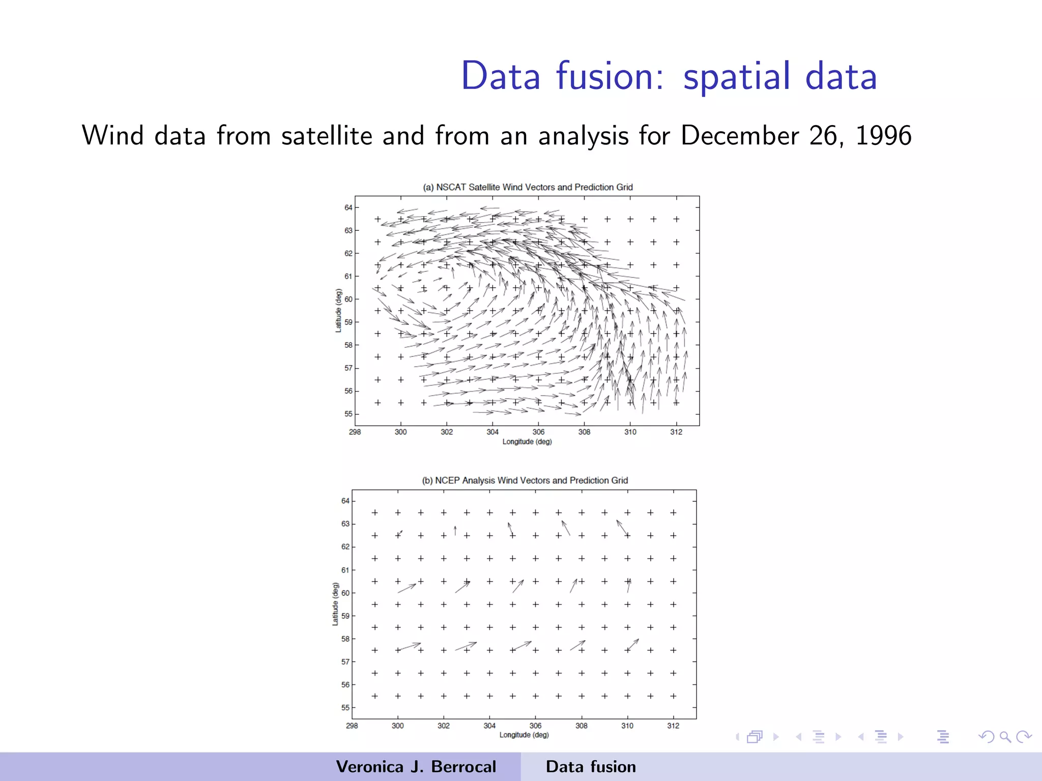
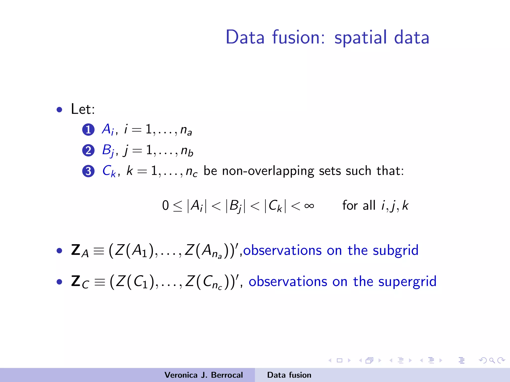
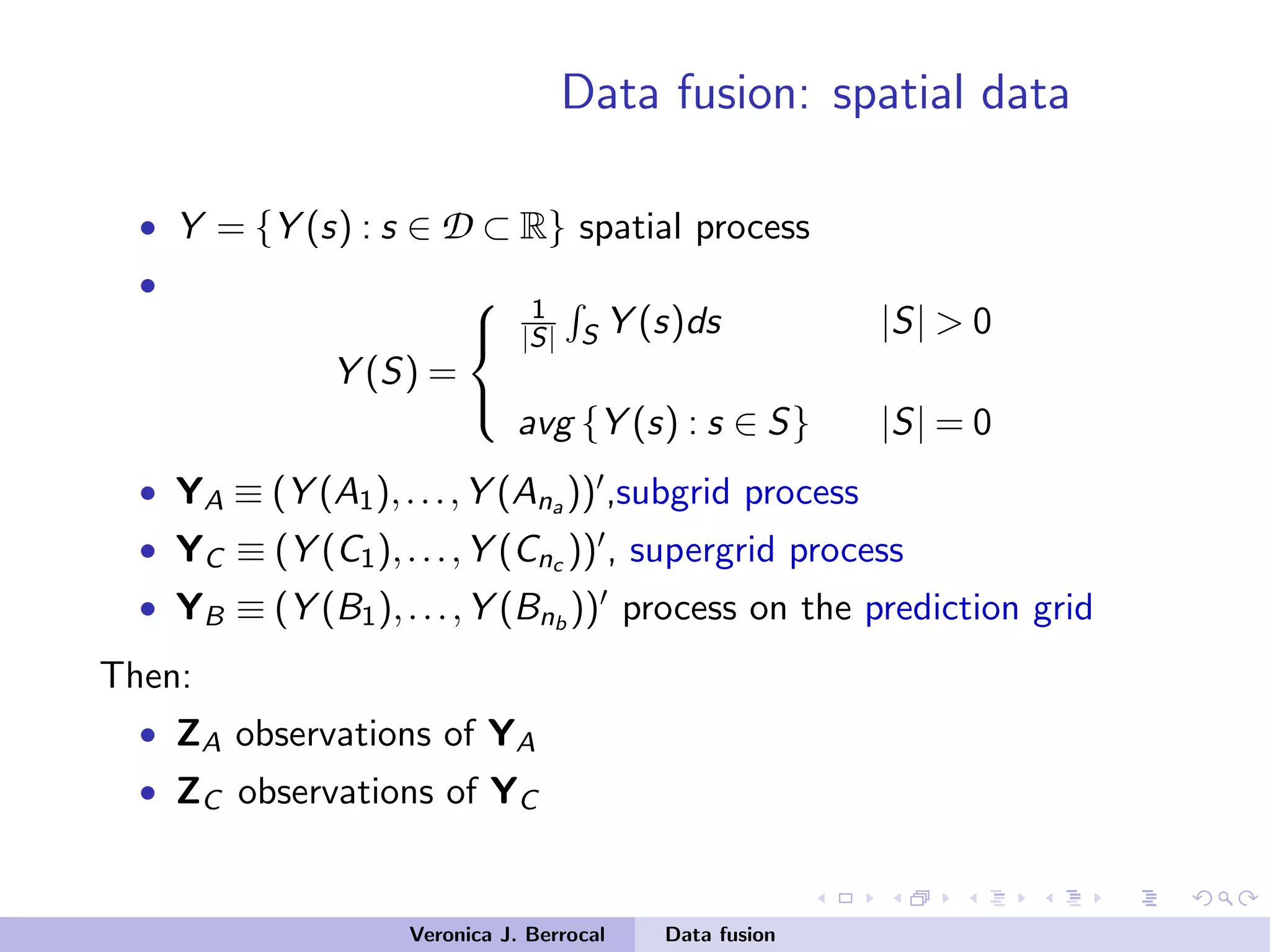
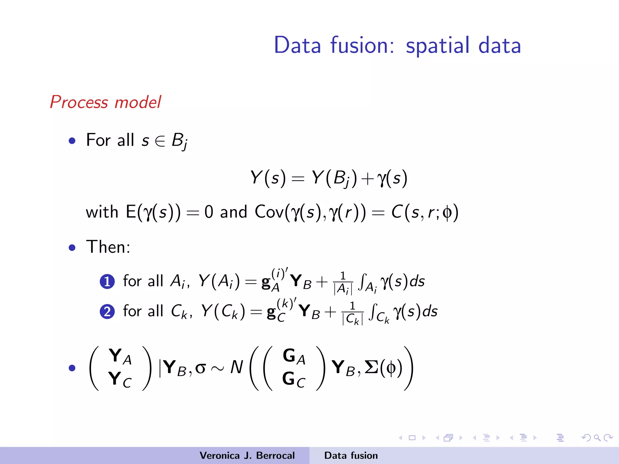
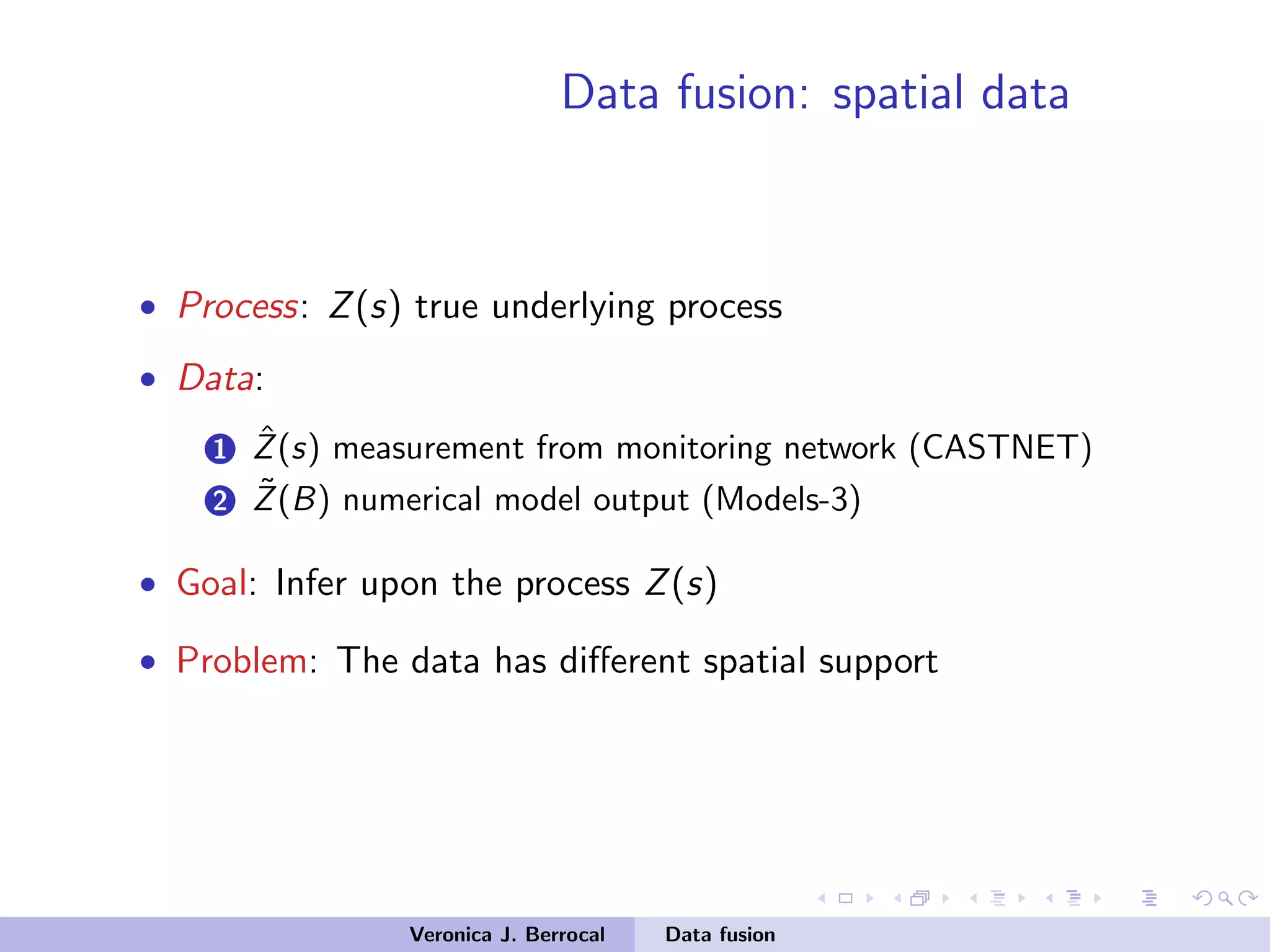
![Data fusion: spatial data
• Z measurement data from the two sources
• Y true underlying process
• Adopt the modeling approach:
[Data Process]
[Process Parameters]
[Parameters]
• Goal: Infer upon the process Y
• Problem: The data has different spatial support
Veronica J. Berrocal Data fusion](https://image.slidesharecdn.com/samsiclass2017berrocal-171004125937/75/CLIM-Fall-2017-Course-Statistics-for-Climate-Research-Guest-lecture-Data-Fusion-Veronica-Berrocal-Sep-26-2017-32-2048.jpg)
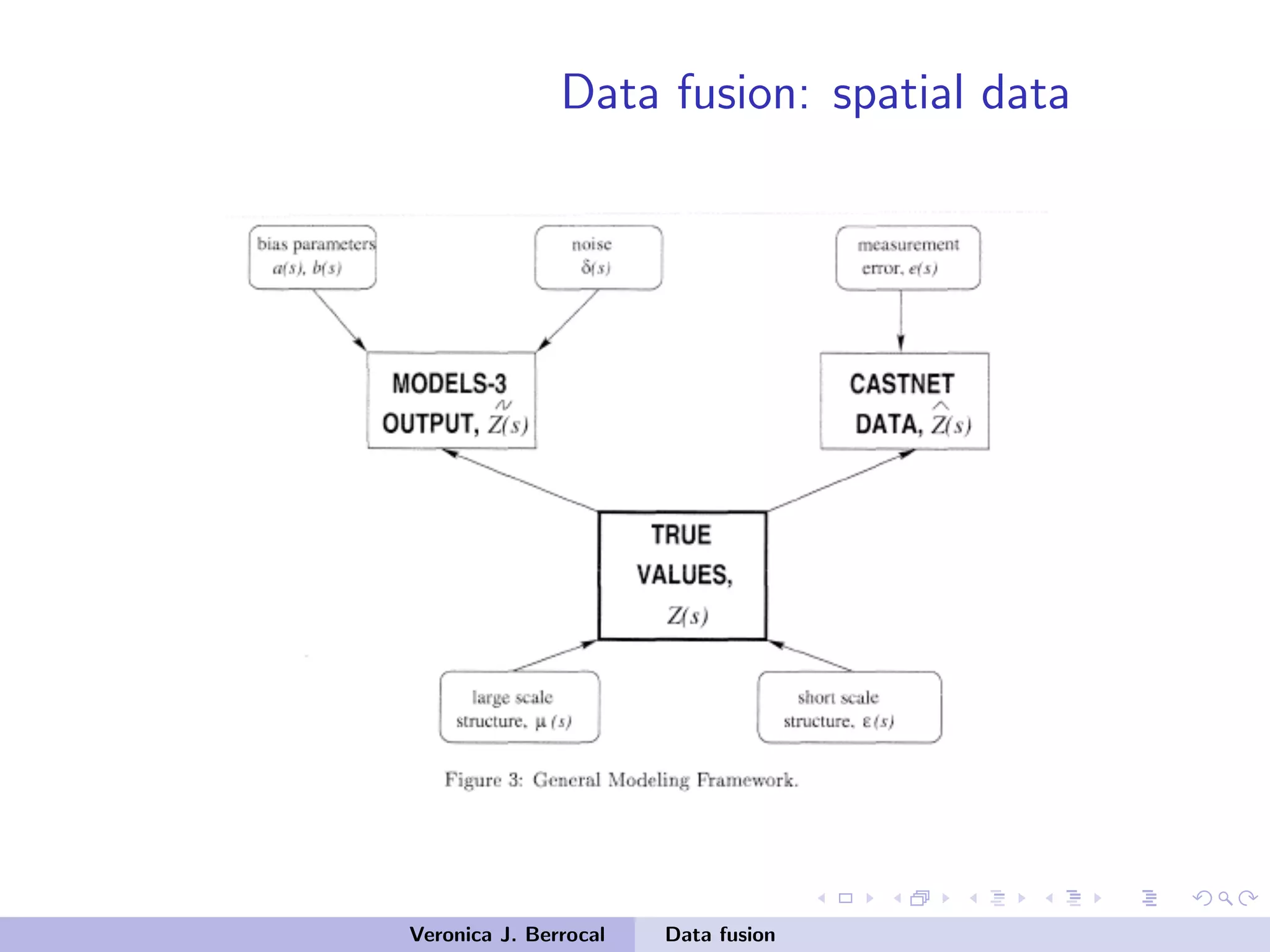
![Data fusion: spatial data
Data model
• Model for [ZA,ZC |YA,YC ,YB,θm]
• Measurement error
ZA = YA +εA εA ∼ N(0, σ2
a Ina )
ZC = YC +εC εC ∼ N(0, σ2
c Inc )
•
ZA
ZC
|YA,YC ,σ2
a,σ2
c ∼
N
YA
YC
,Σm =
σ2
aIna 0
0 σ2
c Inc
Veronica J. Berrocal Data fusion](https://image.slidesharecdn.com/samsiclass2017berrocal-171004125937/75/CLIM-Fall-2017-Course-Statistics-for-Climate-Research-Guest-lecture-Data-Fusion-Veronica-Berrocal-Sep-26-2017-35-2048.jpg)
![Data fusion: spatial data
Complete model
• Data model:
ZA
ZC
|YB,Σm,Σ ∼ N
GA
GC
YB,Σm +Σ(φ)
• Process model: YB ∼ N(θB,ΣB()φ)
• Parameters: [σ2
a,σ2
c,θB,φ]
Veronica J. Berrocal Data fusion](https://image.slidesharecdn.com/samsiclass2017berrocal-171004125937/75/CLIM-Fall-2017-Course-Statistics-for-Climate-Research-Guest-lecture-Data-Fusion-Veronica-Berrocal-Sep-26-2017-37-2048.jpg)
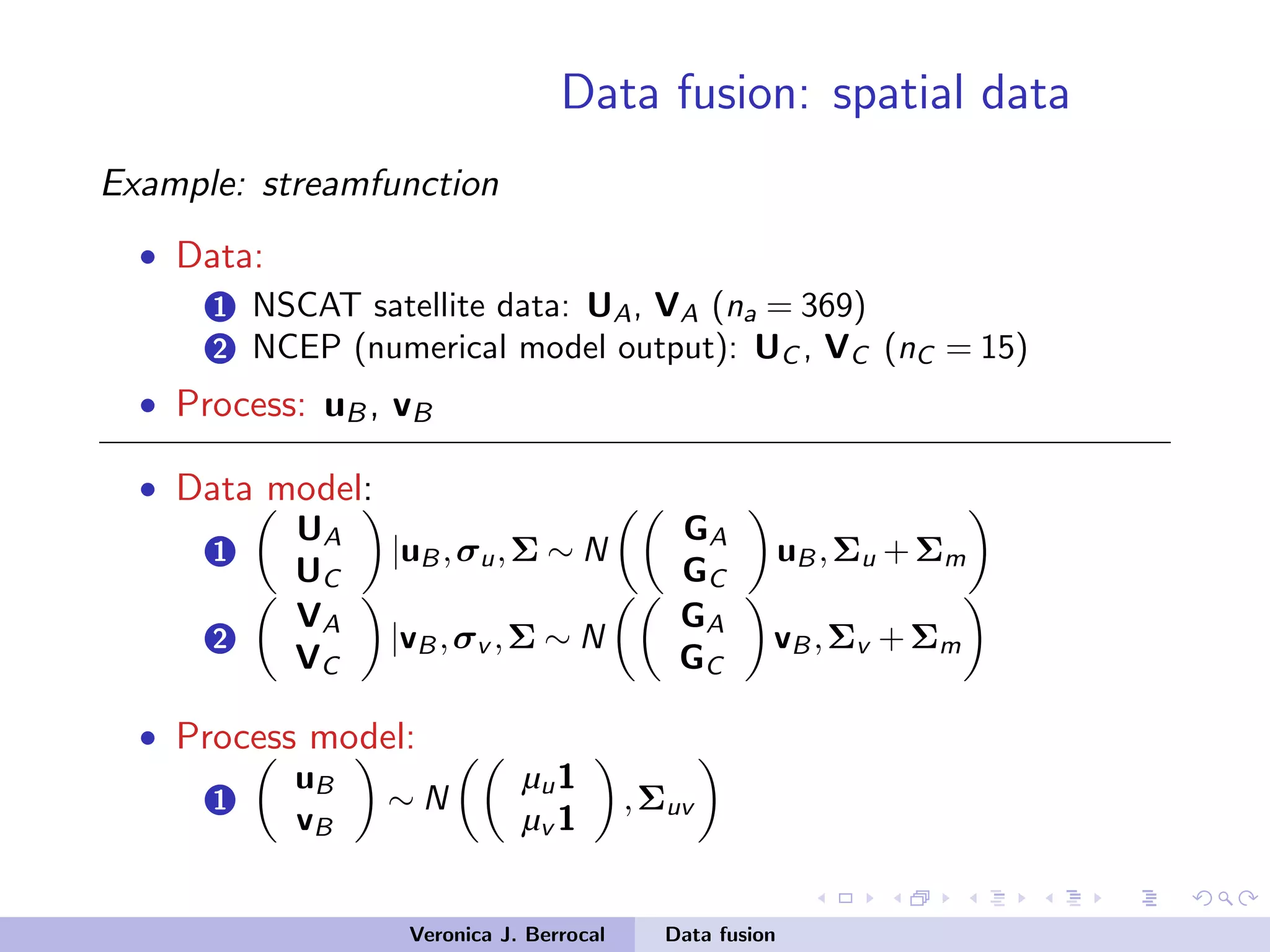
![Data fusion: spatial data
• Interest in predicting the streamfunction ψ.
• Deterministic Poisson equation to determine streamfunction ψ
from winds:
∇2
ψ =
∂v
∂x
−
∂u
∂y
u: east-west wind component, v: north-south wind
component
• Discretizing to a regular grid:
1 ψI |ψbc,u,v ∼ N(L−1
[Dx v −Dy u+Lbc ψbc],ΣI )
2 ψbc ∼ N(µbc ,Σbc )
• ψI : streamfunction at the interior grid locations
• ψbc: streamfunction at the boundary grid locations
Veronica J. Berrocal Data fusion](https://image.slidesharecdn.com/samsiclass2017berrocal-171004125937/75/CLIM-Fall-2017-Course-Statistics-for-Climate-Research-Guest-lecture-Data-Fusion-Veronica-Berrocal-Sep-26-2017-39-2048.jpg)
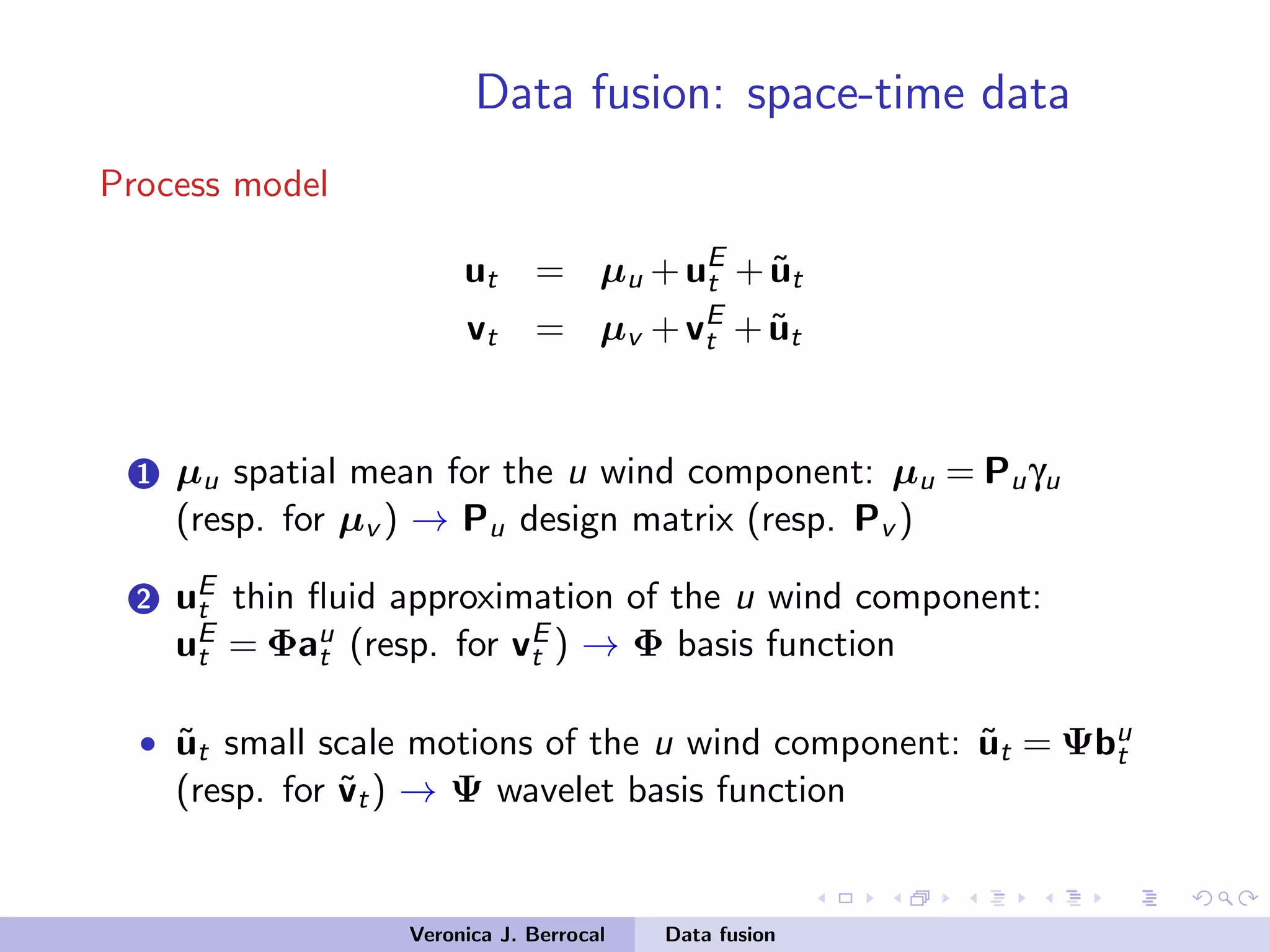
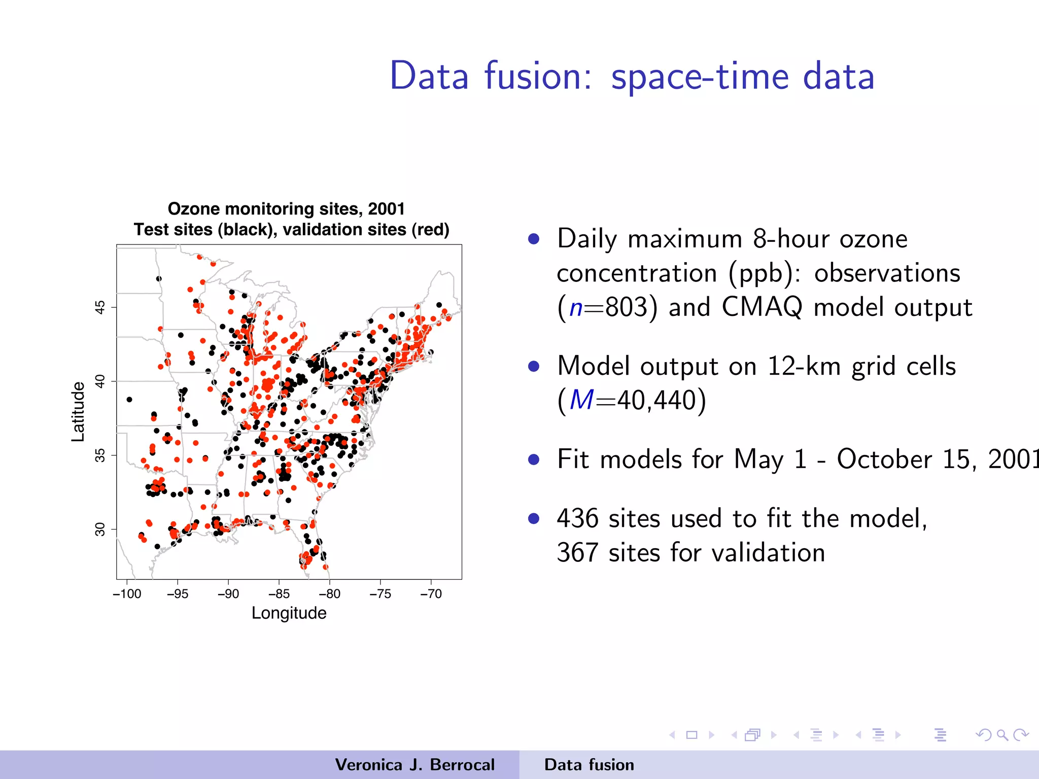
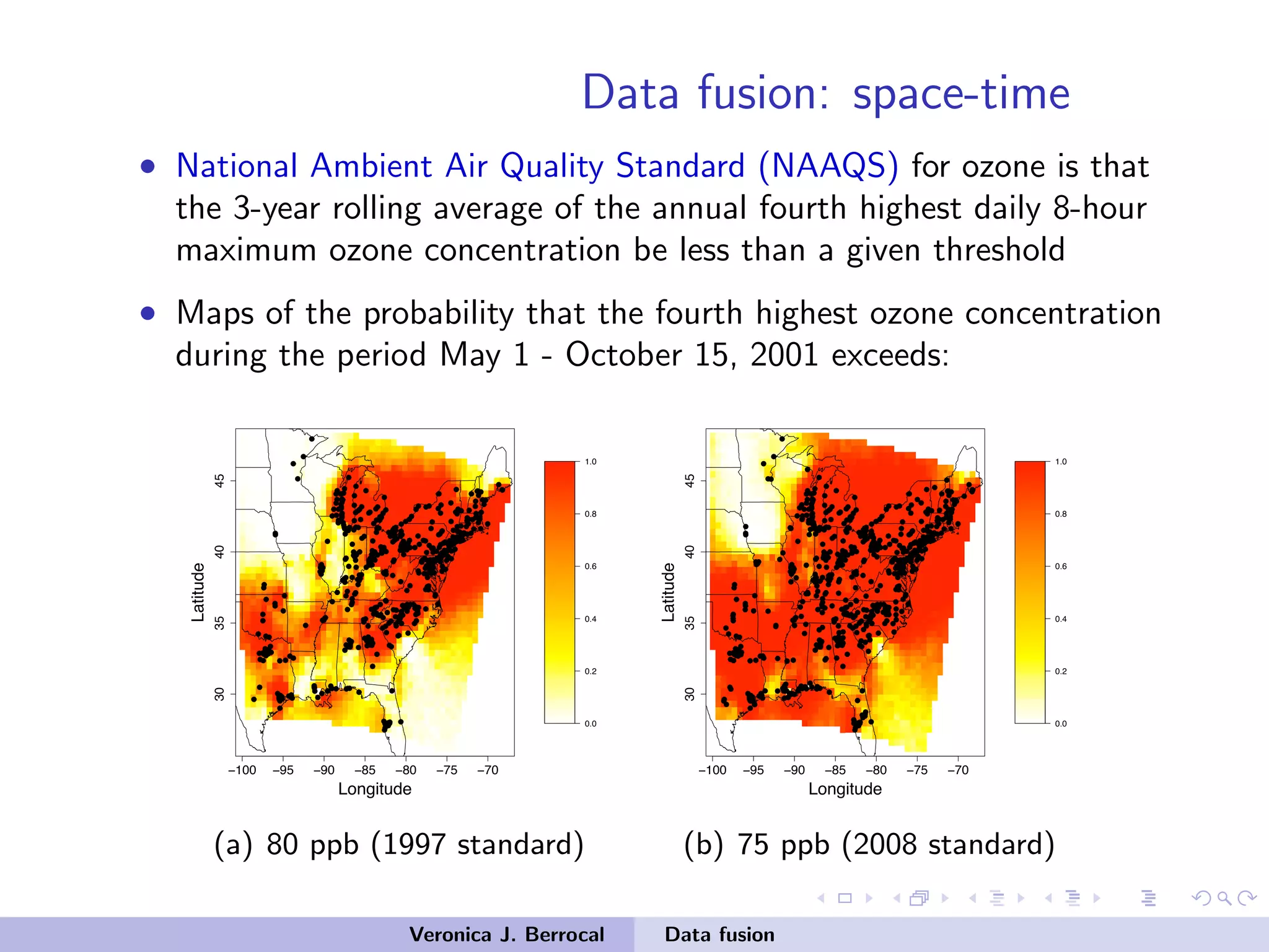
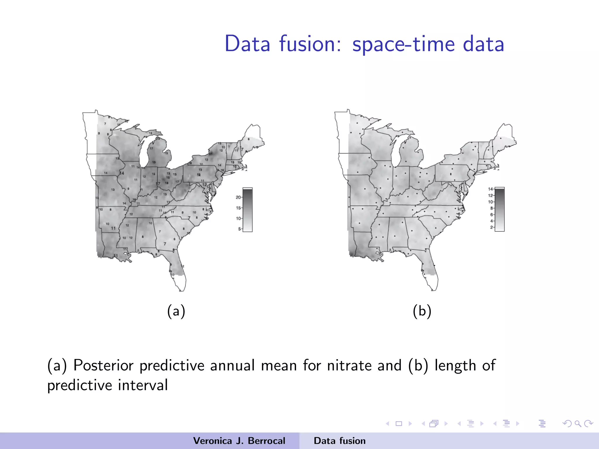
![Data fusion: space-time data
Data model
{V}T
t=1 ,{U}T
t=1 | {v}T
t=1 ,{u}T
t=1 ,θ =
T
∏
t=1
[Vt | vt,θ]·[Ut | ut,θ]
• Vt | vt,Σt ∼ N(Ktvt,Σt)
• Ut | ut,Σt ∼ N(Ktut,Σt)
1 Σt diagonal matrix with entries equal to either σ2
(satellite
obs), σ2
b (NCEP boundary grid cells) or σ2
I (NCEP interior
cells)
2 Kt design matrices that maps the prediction grid cells to the
observation grid cells
Veronica J. Berrocal Data fusion](https://image.slidesharecdn.com/samsiclass2017berrocal-171004125937/75/CLIM-Fall-2017-Course-Statistics-for-Climate-Research-Guest-lecture-Data-Fusion-Veronica-Berrocal-Sep-26-2017-53-2048.jpg)
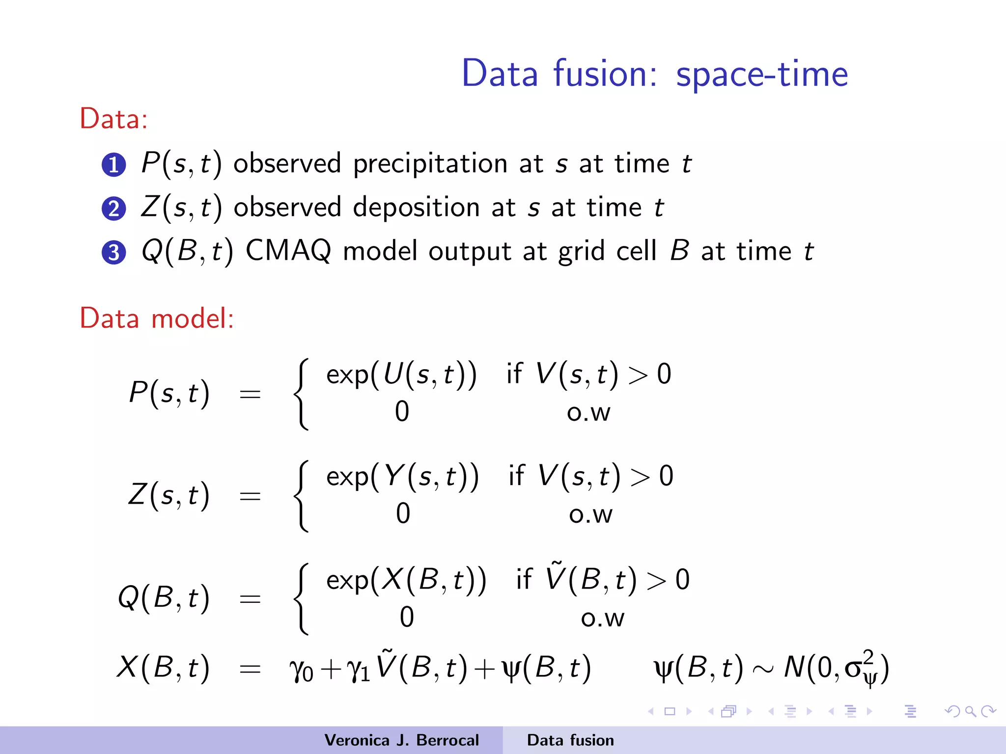
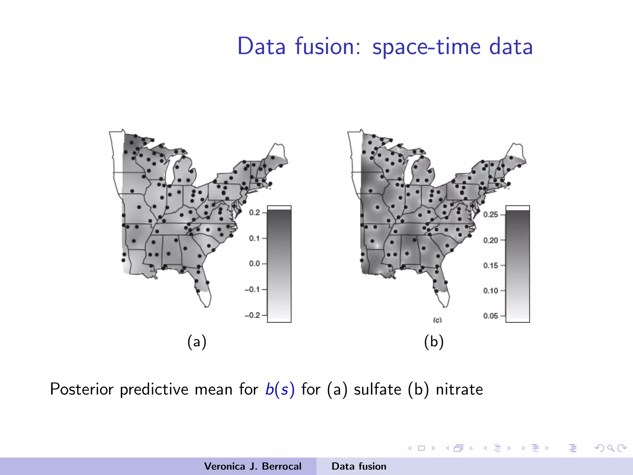
![Data fusion: space-time data
Data model
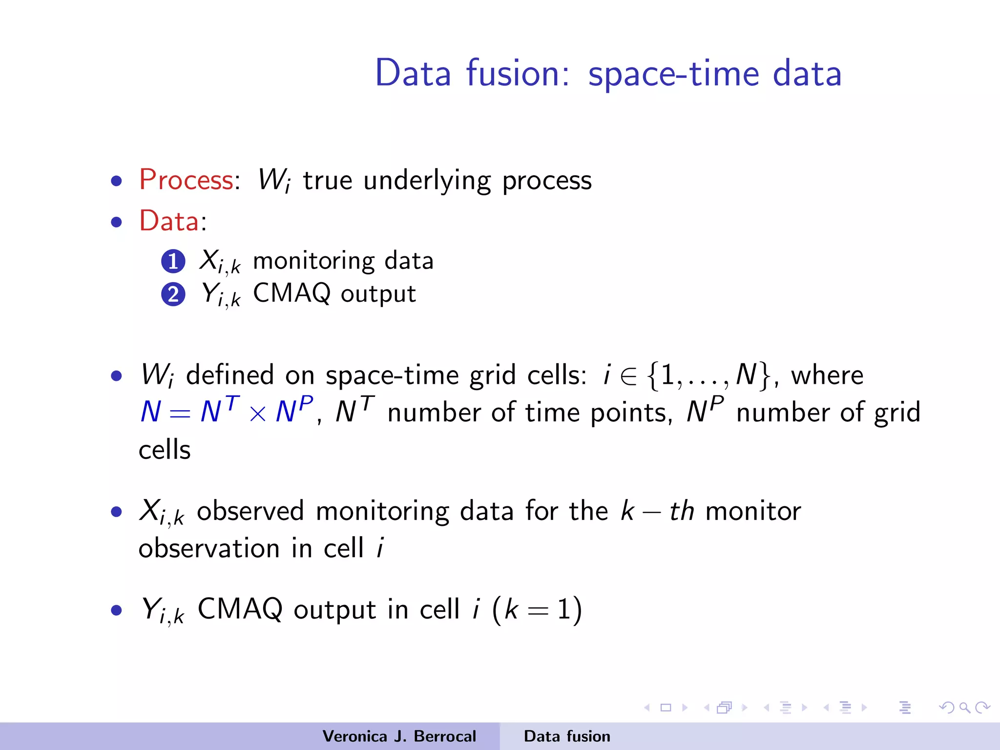
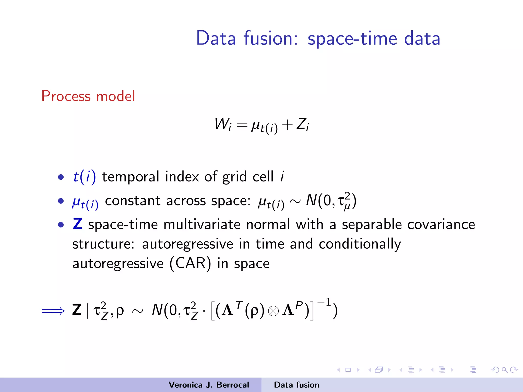
• Model for [Xi,k,Yi,k | Wi ,θ]
Measurement error
Xi,k = Wi +εi,k εi,k ∼ N(0,τ2
X )
Yi,k = Di β +Wi +δi,k δi,k ∼ N(0,τ2
Y )
• Di : vector of uniform B-splines over a regular 3-dimensional
lattice of ND knots
=⇒ CMAQ bias for grid cell i : Di β = ∑ND
j=1 Dij βj
Veronica J. Berrocal Data fusion](https://image.slidesharecdn.com/samsiclass2017berrocal-171004125937/75/CLIM-Fall-2017-Course-Statistics-for-Climate-Research-Guest-lecture-Data-Fusion-Veronica-Berrocal-Sep-26-2017-61-2048.jpg)
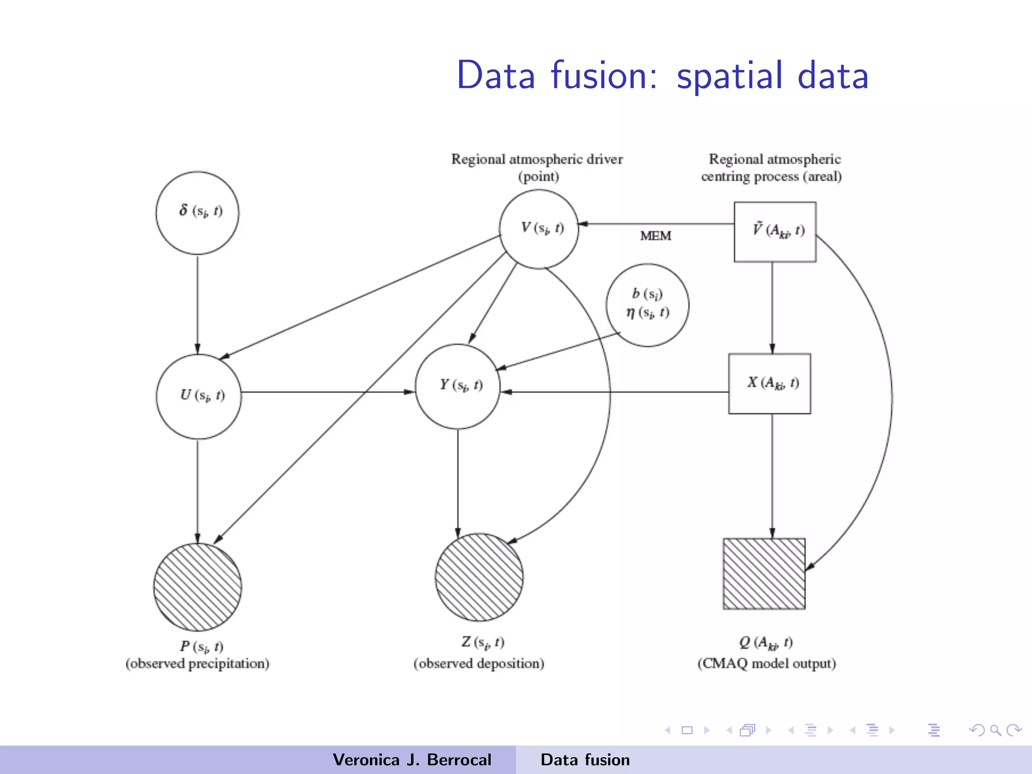
![Data fusion: space-time
Process model:
1 U(s,t) process driving precipitation at s at time t
2 Y (s,t) process driving deposition at s at time t
3 V (s,t) latent atmospheric process
4 ˜V (B,t) process driving the log-CMAQ output at B at time t
U(s,t) = α0 +α1V (s,t)+δ(s,t) δt ∼ GP(0,Σδ)
Y (s,t) = β0 +β1U(s,t)+β2V (s,t)+[b0 +b1(s)X(B,t)]+η(s,t)+ε(s,t)
V (s,t) = ˜V (B,t)+ν(s,t) ν(s,t) ∼ N(0,σ2
ψ)
˜V (B,t) = ρ ˜V (B,t −1)+ζ(B,t) ζ(B,t) ∼ CAR
Veronica J. Berrocal Data fusion](https://image.slidesharecdn.com/samsiclass2017berrocal-171004125937/75/CLIM-Fall-2017-Course-Statistics-for-Climate-Research-Guest-lecture-Data-Fusion-Veronica-Berrocal-Sep-26-2017-88-2048.jpg)
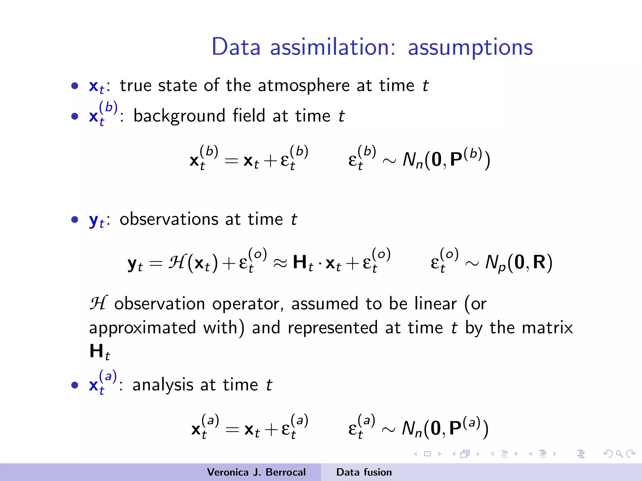
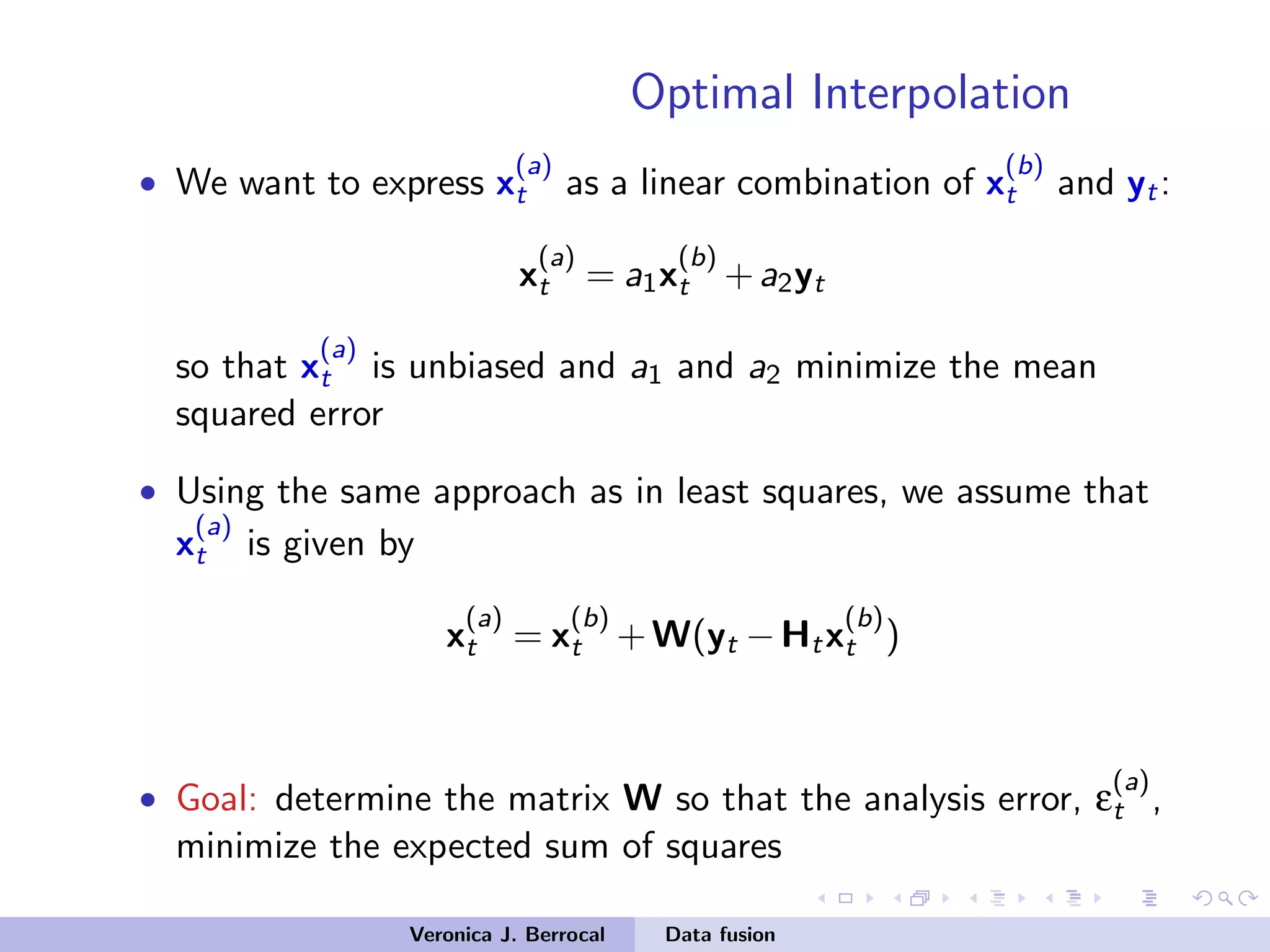
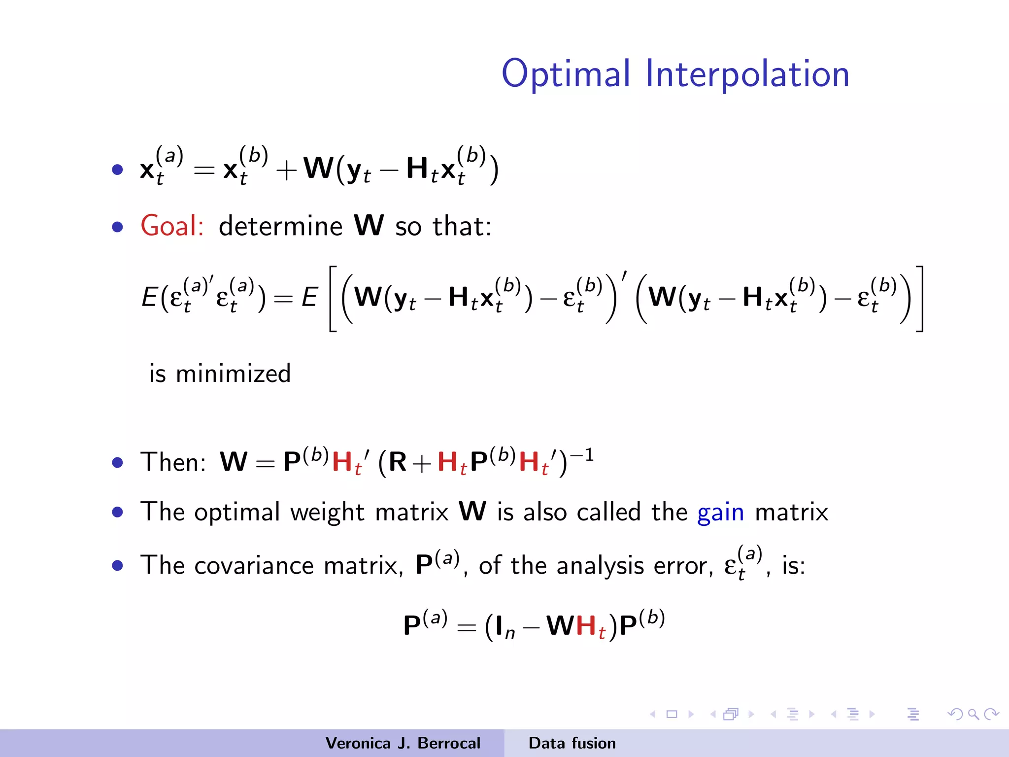
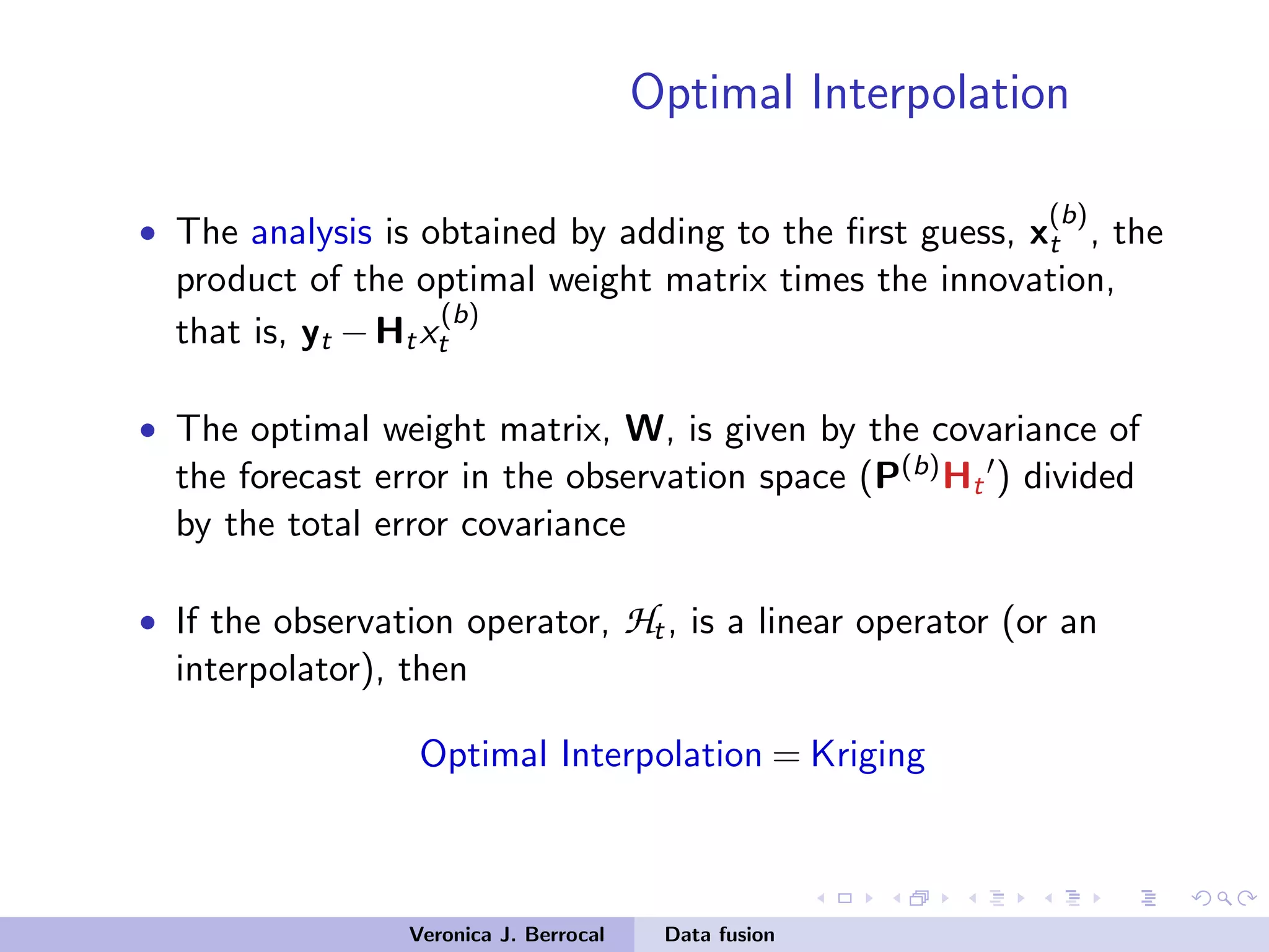
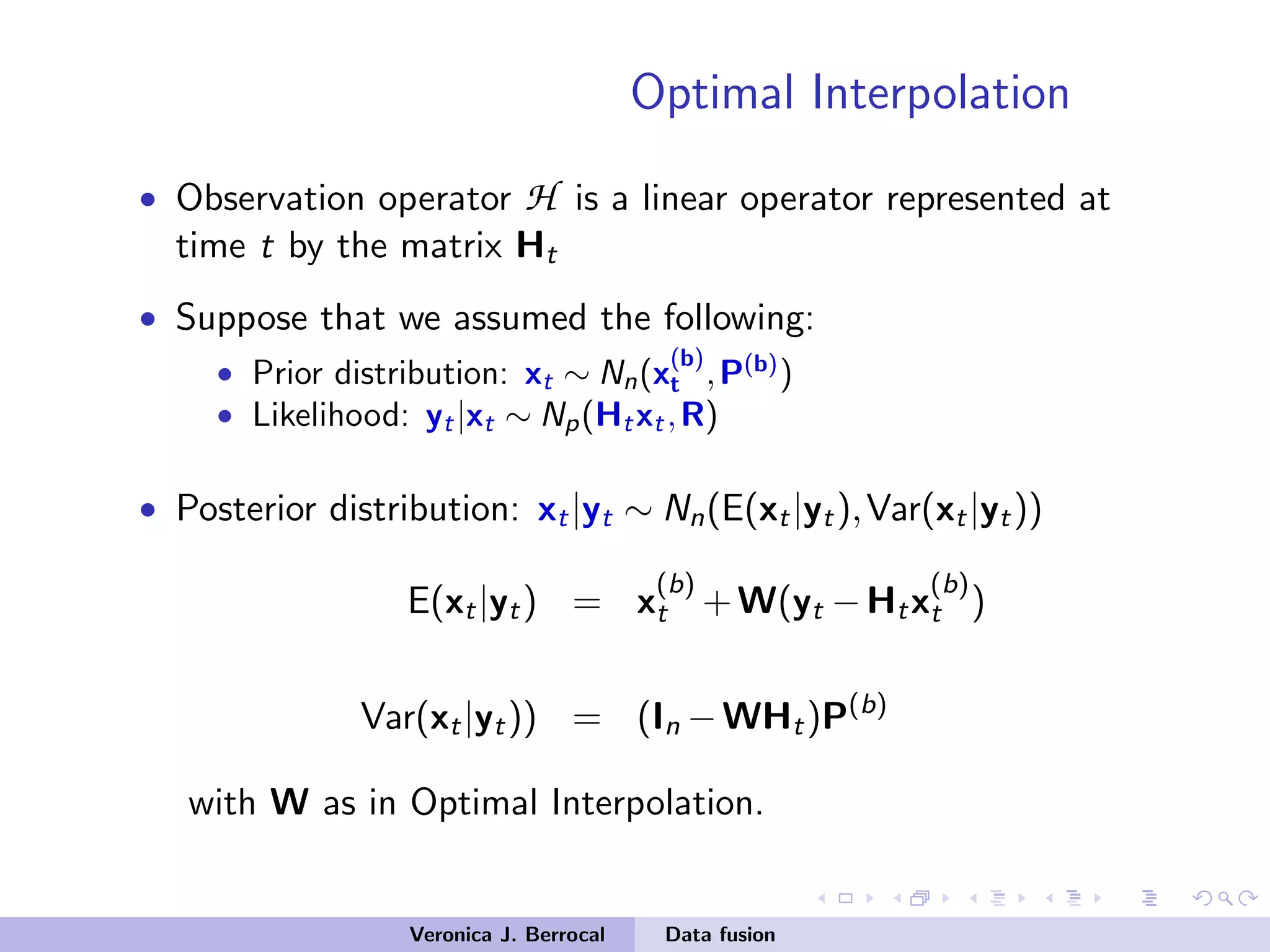
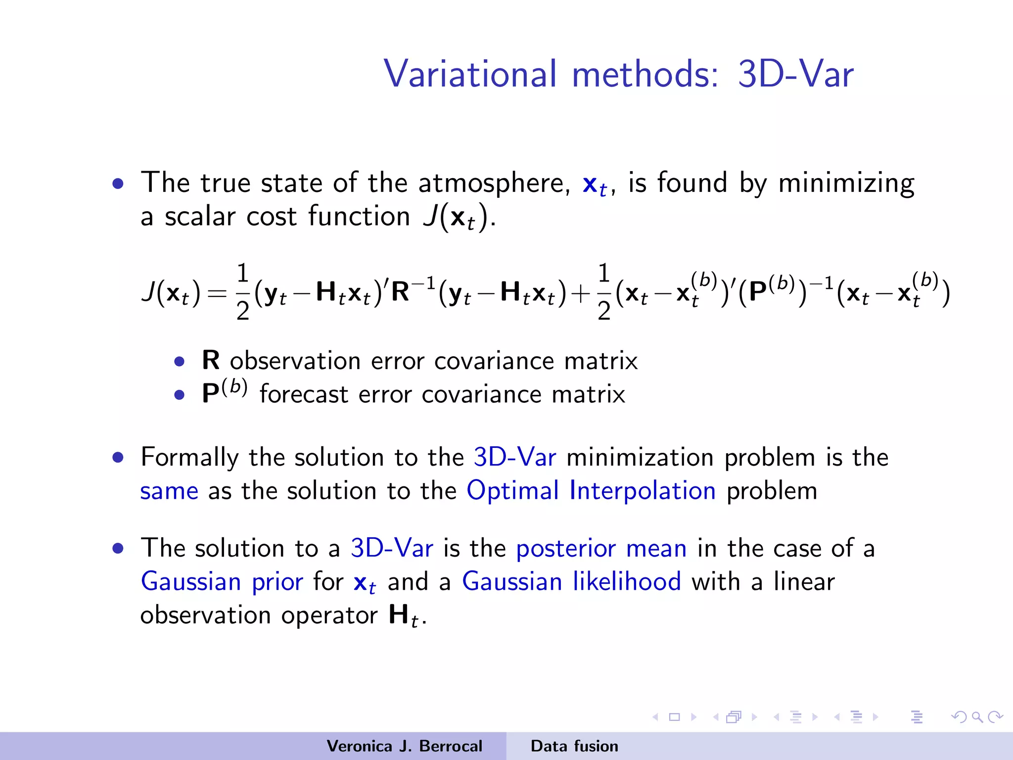
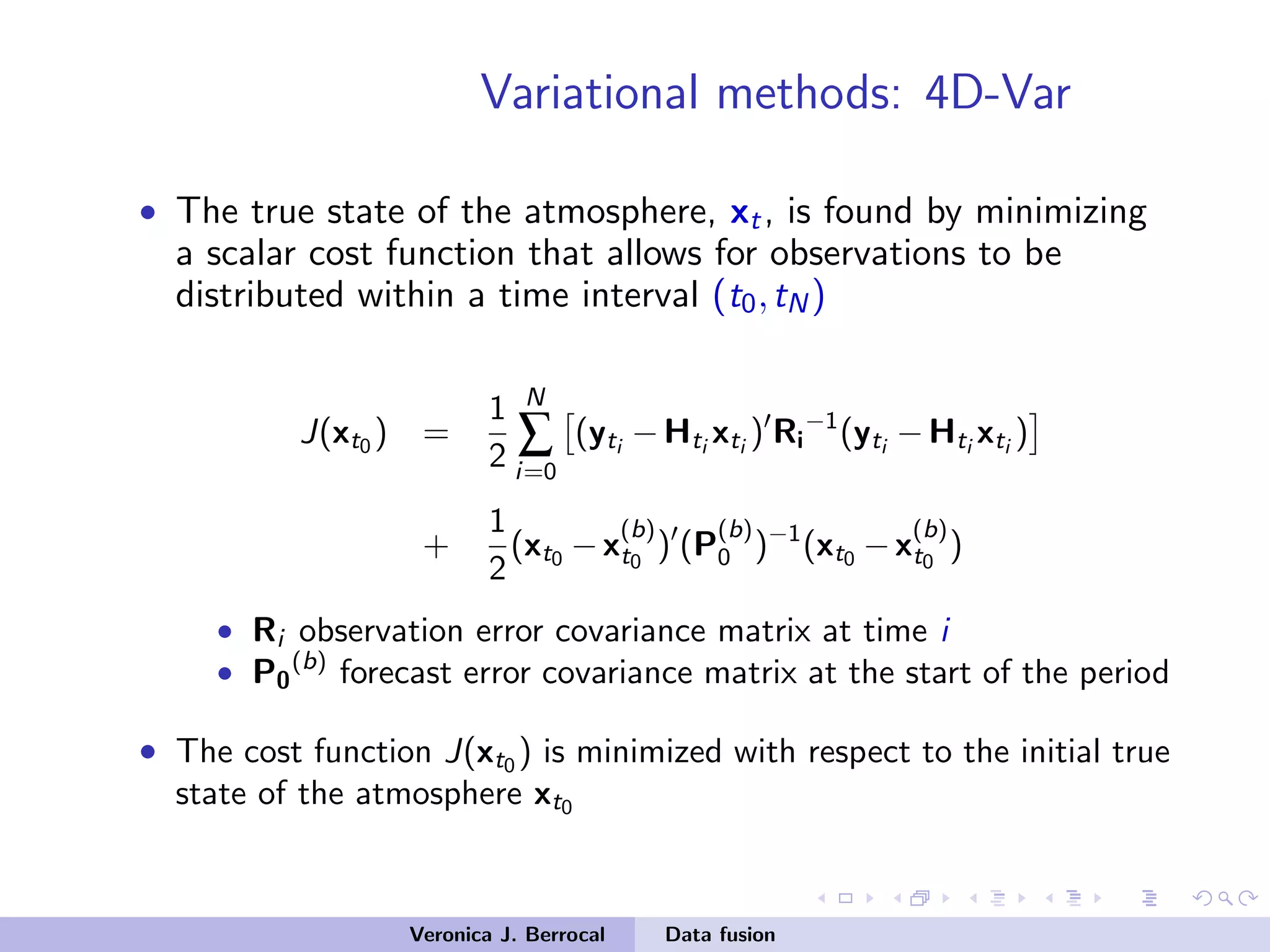
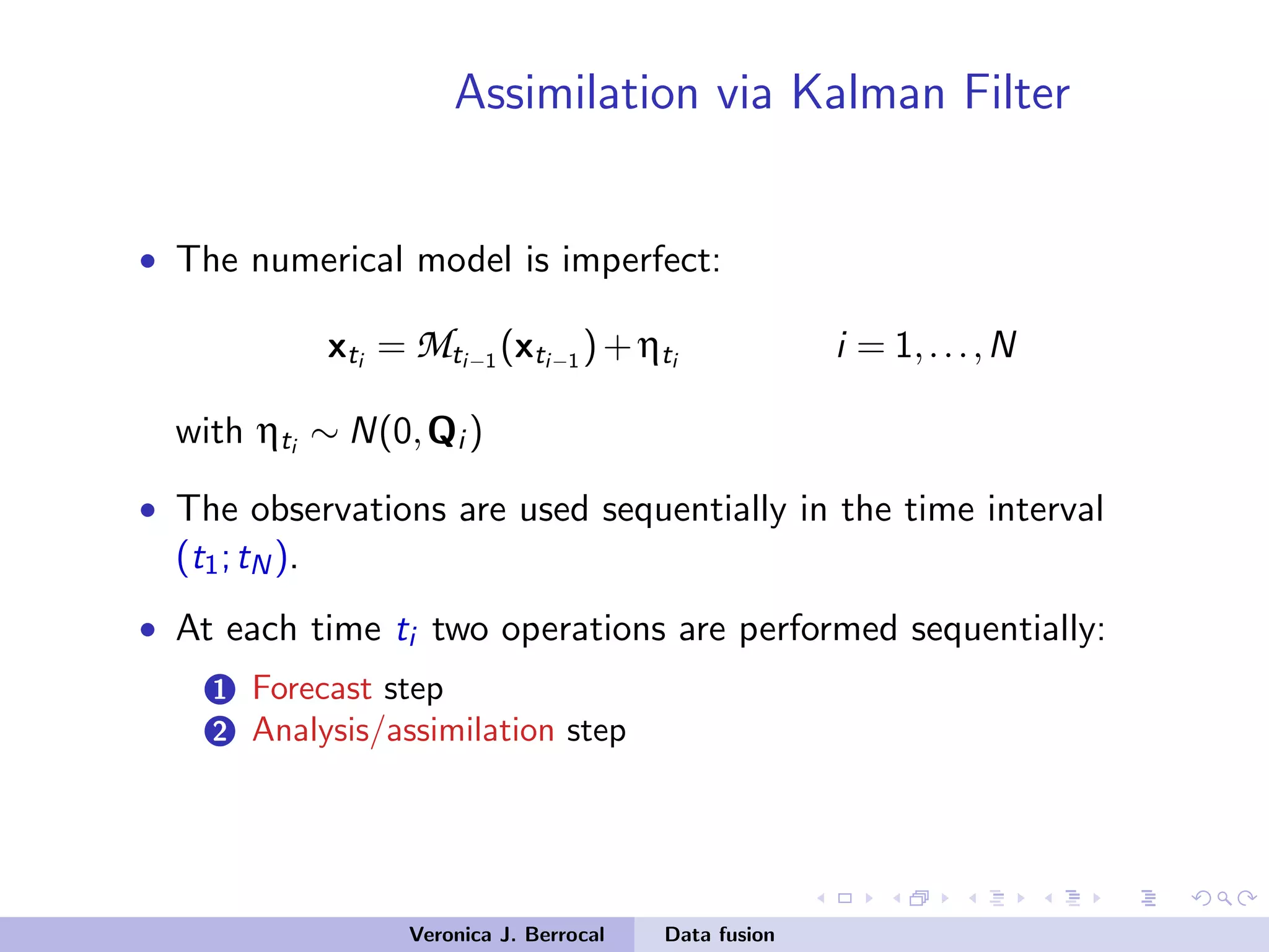
This document discusses various approaches for data fusion, which refers to statistically combining data from different sources. The main approaches covered are data assimilation, optimal interpolation, variational methods, and the Kalman filter. Data assimilation aims to combine model output with observations to estimate the true state. Optimal interpolation finds the best linear combination of a background field and observations to minimize error. Variational methods determine the state by minimizing a cost function, while the Kalman filter sequentially assimilates observations using forecast and analysis steps. The goal of all these approaches is to integrate multiple data sources to obtain a better estimate of the true state than using any one source alone.