This document discusses the relationship between difference-in-differences (DiD) and lagged-dependent-variable (LDV) adjustment methods in causal inference. It presents a framework for identifying causal effects and highlights the importance of the assumptions underlying these methodologies, including parallel trends and stationarity. The findings suggest conditions under which DiD estimates may overestimate or underestimate true causal effects, with examples illustrating these concepts in real-world studies.

1. A bracketing relationship between
difference-in-differences and
lagged-dependent-variable adjustment
Peng Ding
UC Berkeley, Statistics
December 10, 2019 at SAMSI
With Fan Li at Duke Statistics, published in Political Analysis
1 / 20

2. Classic Card and Krueger (1994)
▶ Minimum wage increased in New Jersey in 1992, not in Pennsylvania
▶ Observed employment in fast food restaurants before and after
▶ Figure from Angrist and Pischke (2008) book:
2 / 20

3. The basic two-period two-group panel design
▶ Units: i = 1, . . . , n
▶ Two periods—“before” and “after”: T = t, t + 1
▶ Two groups—control and treatment: Gi = 0, 1
▶ Treatment is only assigned to group Gi = 1 in the “after” period
▶ DiT : the observed treatment status at time T
▶ Dit ≡ 0 (all control in the “before” period)
▶ Di,t+1 = 1 for the units in group Gi = 1 =⇒ Gi = Di,t+1
▶ Outcome YiT : i = 1, . . . , n and T = t, t + 1
3 / 20

4. Potential outcomes and causal effects
▶ Potential outcomes {YiT (1), YiT (0)}
▶ Observed outcomes: YiT = YiT (DiT )
before T = t after T = t + 1
control group G = 0 Yit = Yit(0) Yi,t+1 = Yi,t+1(0)
treatment group G = 1 Yit = Yit(0) Yi,t+1 = Yi,t+1(1)
▶ Causal estimand — average effect on the treated:
τATT = E{Yi,t+1(1) − Yi,t+1(0) | Gi = 1} = µ1 − µ0
▶ µ1 = E{Yi,t+1(1) | Gi = 1} = E(Yi,t+1 | Gi = 1) identifiable
▶ µ0 = E{Yi,t+1(0) | Gi = 1}: counterfactual
▶ key: inferring µ0 based on observables 4 / 20

5. Difference-in-differences (DID)
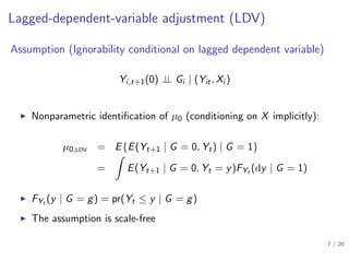
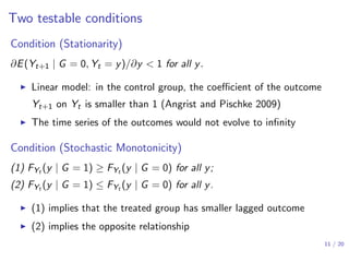
Assumption (Parallel trends conditioning on covariates Xi )
E{Yi,t+1(0) − Yi,t(0) | Xi , Gi = 1} = E{Yi,t+1(0) − Yi,t(0) | Xi , Gi = 0}
▶ Nonparametric identification of µ0 = E{Yi,t+1(0) | Gi = 1}
µ0,DID = E [E{Yit (0) | Xi , Gi = 1} + E{Yi,t+1(0) − Yit (0) | Xi , Gi = 0} | Gi = 1]
= E(Yit | Gi = 1) + E{E(Yi,t+1 − Yit | Xi , Gi = 0) | Gi = 1}
▶ Without covariates — difference-in-difference
▶ nonparametric identification:
µ0 = E(Yit | Gi = 1) + E(Yi,t+1 | Gi = 0) − E(Yit | Gi = 0)
▶ moment estimator: ˆτDID = ( ¯Y1,t+1 − ¯Y1,t) − ( ¯Y0,t+1 − ¯Y0,t)
5 / 20

6. The scale dependent issue of DID
▶ Parallel trends may hold for the original Y but not for a nonlinear
monotone transformation of Y , for example, log Y
▶ This restricts the use of DID in general settings
▶ Athey and Imbens (2006): “parallel trends” on the CDF level
▶ Sofer et al. (2016): an negative outcome control approach
6 / 20

7. Lagged-dependent-variable adjustment (LDV)
Assumption (Ignorability conditional on lagged dependent variable)
Yi,t+1(0) ⊥⊥ Gi | (Yit, Xi )
▶ Nonparametric identification of µ0 (conditioning on X implicitly):
µ0,LDV = E{E(Yt+1 | G = 0, Yt) | G = 1}
=
∫
E(Yt+1 | G = 0, Yt = y)FYt (dy | G = 1)
▶ FYt (y | G = g) = pr(Yt ≤ y | G = g)
▶ The assumption is scale-free
7 / 20

8. A bracketing relationship based on linear model fitting
a little more general than Angrist and Pischke (2009)
▶ Ignore covariates X
▶ Two versions of LDV
▶ fit ˆE(Yt+1 | G = 0, Yt = y) = ˆα + ˆβYt under control:
ˆτLDV = ( ¯Y1,t+1 − ¯Y0,t+1) − ˆβ( ¯Y1,t − ¯Y0,t)
▶ fit ˆE(Yt+1 | G, Yt) = ˆα + ˆτ′
LDVG + ˆβ′
Yt using all units:
ˆτ′
LDV = ( ¯Y1,t+1 − ¯Y0,t+1) − ˆβ′
( ¯Y1,t − ¯Y0,t)
▶ Compared to DID
ˆτDID = ( ¯Y1,t+1 − ¯Y0,t+1) − ( ¯Y1,t − ¯Y0,t)
8 / 20

9. Interpreting the bracketing relationship under linear models
▶ Consider the case with ˆβ or ˆβ′ smaller than 1
▶ The sign of ˆτDID − ˆτLDV or ˆτDID − ˆτ′
LDV depends on the sign of ¯Y1,t − ¯Y0,t
▶ Treatment group has smaller Yt on average =⇒ ˆτDID > ˆτLDV
▶ Treatment group has larger Yt on average =⇒ ˆτDID < ˆτLDV
▶ How much ˆβ or ˆβ′ deviates from 1
=⇒ how different the DID and LDV estimates are
▶ They are identical if ˆβ = 1 or ˆβ′ = 1
9 / 20

10. A lemma: conditioning on X implicitly
Lemma
The difference between µ0,DID and µ0,LDV is
µ0,LDV − µ0,DID =
∫
∆(y)FYt (dy | G = 1) −
∫
∆(y)FYt (dy | G = 0)
▶ Depends on average changed outcome given Yt in control group:
∆(y) = E(Yt+1 | G = 0, Yt = y) − y
= E(Yt+1 − Yt | G = 0, Yt = y)
▶ Depends on the difference between the distribution of Yt in the
treated and control groups
10 / 20

11. Two testable conditions
Condition (Stationarity)
∂E(Yt+1 | G = 0, Yt = y)/∂y < 1 for all y.
▶ Linear model: in the control group, the coefficient of the outcome
Yt+1 on Yt is smaller than 1 (Angrist and Pischke 2009)
▶ The time series of the outcomes would not evolve to infinity
Condition (Stochastic Monotonicity)
(1) FYt (y | G = 1) ≥ FYt (y | G = 0) for all y;
(2) FYt (y | G = 1) ≤ FYt (y | G = 0) for all y.
▶ (1) implies that the treated group has smaller lagged outcome
▶ (2) implies the opposite relationship
11 / 20

12. A theorem
Theorem
If Stationarity and Stochastic Monotonicity(1) hold, then
µ0,DID ≤ µ0,LDV, τDID ≥ τLDV.
If Stationarity and Stochastic Monotonicity(2) hold, then
µ0,DID ≥ µ0,LDV, τDID ≤ τLDV.
▶ It does not require the parallel trends or the ignorability
▶ Simply a result on the relative magnitude between τDID and τLDV
▶ Extends Angrist and Pischke (2009) to the nonparametric setting
12 / 20

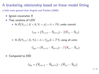
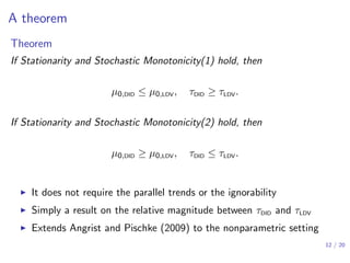
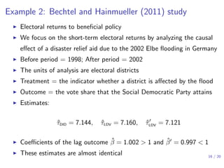
13. Interpretations of the theorem
▶ Under Stationarity and Stochastic Monotonicity(1),
τDID ≥ τLDV
▶ Both of them can be biased for the true causal effect τATT
▶ τDID ≥ τLDV ≥ τATT =⇒ τDID over-estimates τATT more than τLDV
▶ τATT ≥ τDID ≥ τLDV =⇒ τLDV under-estimates τATT more than τDID
▶ τDID ≥ τATT ≥ τLDV =⇒ τDID and τLDV are the upper and lower bounds
▶ In the last case, [τLDV, τDID] bracket the true causal effect
▶ Analogous results under Stationarity and Stochastic Monotonicity(2)
13 / 20

14. Example 1: Card and Krueger (1994) study
▶ Effect of a minimum wage increase on employment
▶ Employment information in New Jersey and Pennsylvania before and
after a minimum wage increase in New Jersey in 1992
▶ Outcome = # employees at each fast food restaurant
▶ Estimates:
ˆτDID = 2.446, ˆτLDV = 0.302, ˆτ′
LDV = 0.865
▶ Coefficients of the lag outcome ˆβ = 0.288 < 1 and ˆβ′ = 0.475 < 1
▶ The same conclusion under a quadratic model
14 / 20

15. Example 1: graphical checks
10 20 30 40 50 60 70
5102030
G = 0
Yt
Yt+1
0 20 40 60
0.00.20.40.60.81.0
Yt
FYt
(y|G)
G=1
G=0
Left: linear and quadratic fitted lines of E(Yt+1 | G = 0, Yt).
Right: FYt (y | G = g) (g = 0, 1) satisfy Stochastic Monotonicity.
15 / 20

16. Example 2: Bechtel and Hainmueller (2011) study
▶ Electoral returns to beneficial policy
▶ We focus on the short-term electoral returns by analyzing the causal
effect of a disaster relief aid due to the 2002 Elbe flooding in Germany
▶ Before period = 1998; After period = 2002
▶ The units of analysis are electoral districts
▶ Treatment = the indicator whether a district is affected by the flood
▶ Outcome = the vote share that the Social Democratic Party attains
▶ Estimates:
ˆτDID = 7.144, ˆτLDV = 7.160, ˆτ′
LDV = 7.121
▶ Coefficients of the lag outcome ˆβ = 1.002 > 1 and ˆβ′ = 0.997 < 1
▶ These estimates are almost identical 16 / 20

17. Example 2: graphical checks
30 40 50 60
2030405060
G = 0
Yt
Yt+1
30 40 50 60
0.00.20.40.60.81.0
Yt
FYt
(y|G)
G=1
G=0
Left: linear fitted lines of E(Yt+1 | G = 0, Yt).
Right: FYt (y | G = g) (g = 0, 1) satisfy Stochastic Monotonicity.
17 / 20

18. Example 3: data
▶ Evaluating the effects of rumble strips on vehicle crashes
▶ Units: n = 1986 road segments in Pennsylvania
▶ Crash counts before (year 2008) and after (year 2012) the intervention
Table: Crash counts (3+ means 3 or more crashes).
(a) control group G = 0 (b) treated group G = 1
Yt+1
0 1 2 3+
Yt
0 789 238 57 18
1 235 95 40 15
2 61 37 11 6
3+ 26 21 4 2
Yt+1
0 1 2 3+
Yt
0 183 39 7 3
1 40 22 5 2
2 16 4 0 1
3+ 2 6 0 1
18 / 20

19. Example 3: results
▶ Stationarity holds for all y = 0, 1, 2, 3+:
ˆE(Yt+1 | G = 0, Yt = y) = .374, .572, .670, .660
▶ Stochastic Monotonicity(1) holds for y = 0, 1, 2, pr(Yt ≤ y | G = g)
(700, .909, .973) for g = 1; (666, .898, .968) for g = 0
▶ Nonparametric estimate of µ0 under ignorability:
ˆµ0,LDV =
∑
y
ˆE(Yt+1 | G = 0, Yt = y)pr(Yt = y | G = 1) = .438
▶ Under the parallel trend: ˆµ0,DID = .395
▶ Matches the theoretical prediction
19 / 20

20. Discussion
▶ Create a super-model that incorporates both DID and LDV
▶ requires multiple time periods: T = t + 1, . . . , t + K
E(Yi,T | Xi , Yi,T−1, Gi ) = αi + λT + βYi,T−1 + τGi + θ⊤
Xi
▶ Nickell (1981) and Hausman–Taylor (1981) identification and
estimation under this model require much stronger assumptions
▶ Practical suggestion
▶ assumptions for DID and LDV: not nested, cannot be validated by data
▶ report results from both approaches
▶ conduct sensitivity analyses allowing for violations of these assumptions
20 / 20