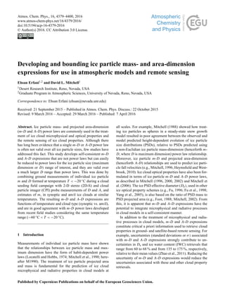
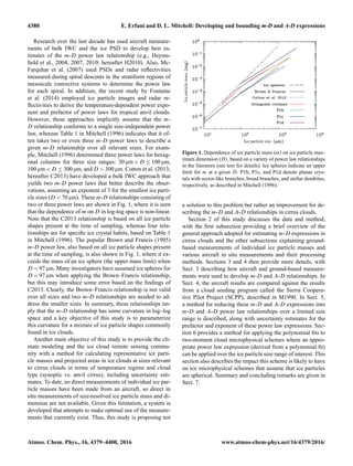
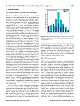
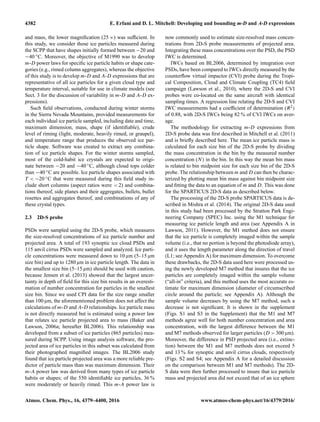
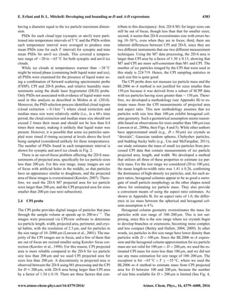
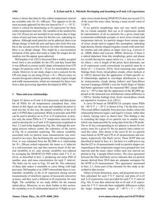
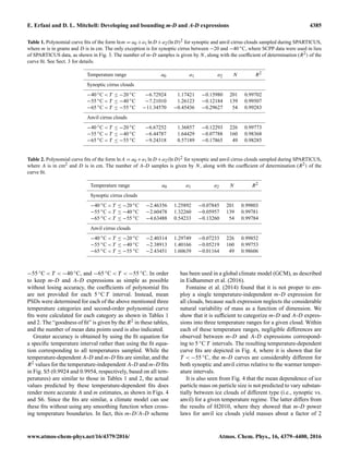
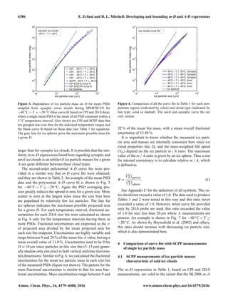
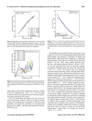
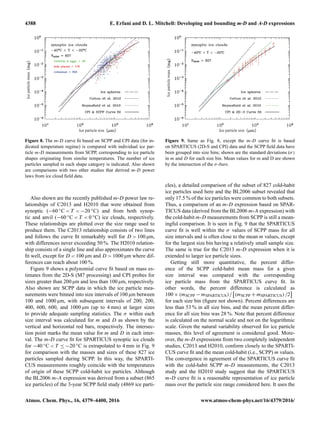
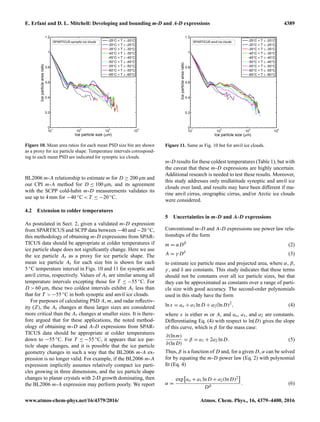
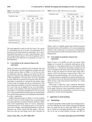
2. 4380 E. Erfani and D. L. Mitchell: Developing and bounding m-D and A-D expressions
Research over the last decade has used aircraft measure-
ments of bulk IWC and the ice PSD to develop best es-
timates of the m-D power law relationship (e.g., Heyms-
field et al., 2004, 2007, 2010; hereafter H2010). Also, Mc-
Farquhar et al. (2007) used PSDs and radar reflectivities
measured during spiral descents in the stratiform regions of
mesoscale convective systems to determine the power law
for each spiral. In addition, the recent study by Fontaine
et al. (2014) employed ice particle images and radar re-
flectivities to derive the temperature-dependent power expo-
nent and prefactor of power laws for tropical anvil clouds.
However, these approaches implicitly assume that the m-
D relationship conforms to a single size-independent power
law, whereas Table 1 in Mitchell (1996) indicates that it of-
ten takes two or even three m-D power laws to describe a
given m-D relationship over all relevant sizes. For exam-
ple, Mitchell (1996) determined three power laws for hexag-
onal columns for three size ranges: 30 µm < D ≤ 100 µm,
100 µm < D ≤ 300 µm, and D > 300 µm. Cotton et al. (2013;
hereafter C2013) have developed a bulk IWC approach that
yields two m-D power laws that better describe the obser-
vations, assuming an exponent of 3 for the smallest ice parti-
cle sizes (D < 70 µm). These m-D relationships consisting of
two or three power laws are shown in Fig. 1, where it is seen
that the dependence of m on D in log-log space is non-linear.
Note that the C2013 relationship is based on all ice particle
shapes present at the time of sampling, whereas four rela-
tionships are for specific ice crystal habits, based on Table 1
in Mitchell (1996). The popular Brown and Francis (1995)
m-D power law, also based on all ice particle shapes present
at the time of sampling, is also shown in Fig. 1, where it ex-
ceeds the mass of an ice sphere (the upper mass limit) when
D < 97 µm. Many investigators have assumed ice spheres for
D < 97 µm when applying the Brown–Francis relationship,
but this may introduce some error based on the findings of
C2013. Clearly, the Brown–Francis relationship is not valid
over all sizes and two m-D relationships are needed to ad-
dress the smaller sizes. In summary, these relationships im-
ply that the m-D relationship has some curvature in log–log
space and a key objective of this study is to parameterize
this curvature for a mixture of ice particle shapes commonly
found in ice clouds.
Another main objective of this study is to provide the cli-
mate modeling and the ice cloud remote sensing commu-
nity with a method for calculating representative ice parti-
cle masses and projected areas in ice clouds at sizes relevant
to cirrus clouds in terms of temperature regime and cloud
type (synoptic vs. anvil cirrus), including uncertainty esti-
mates. To date, no direct measurements of individual ice par-
ticle masses have been made from an aircraft, so direct in
situ measurements of size-resolved ice particle mass and di-
mension are not available. Given this limitation, a system is
developed that attempts to make optimal use of the measure-
ments that currently exist. Thus, this study is proposing not
Figure 1. Dependence of ice particle mass (m) on ice particle max-
imum dimension (D), based on a variety of power law relationships
in the literature (see text for details). Ice spheres indicate an upper
limit for m at a given D. P1b, P1c, and P1d denote planar crys-
tals with sector-like branches, broad branches, and stellar dendrites,
respectively, as described in Mitchell (1996).
a solution to this problem but rather an improvement for de-
scribing the m-D and A-D relationships in cirrus clouds.
Section 2 of this study discusses the data and method,
with the first subsection providing a brief overview of the
general approach adopted for estimating m-D expressions in
cirrus clouds and the other subsections explaining ground-
based measurements of individual ice particle masses and
various aircraft in situ measurements and their processing
methods. Sections 3 and 4 then provide more details, with
Sect. 3 describing how aircraft and ground-based measure-
ments were used to develop m-D and A-D relationships. In
Sect. 4, the aircraft results are compared against the results
from a cloud seeding program called the Sierra Coopera-
tive Pilot Project (SCPP), described in M1990. In Sect. 5,
a method for reducing these m-D and A-D expressions into
m-D and A-D power law relationships over a limited size
range is described, along with uncertainty estimates for the
prefactor and exponent of these power law expressions. Sec-
tion 6 provides a method for applying the polynomial fits to
two-moment cloud microphysical schemes where an appro-
priate power law expression (derived from a polynomial fit)
can be applied over the ice particle size range of interest. This
section also describes the impact this scheme is likely to have
on ice microphysical schemes that assume that ice particles
are spherical. Summary and concluding remarks are given in
Sect. 7.
Atmos. Chem. Phys., 16, 4379–4400, 2016 www.atmos-chem-phys.net/16/4379/2016/
3. E. Erfani and D. L. Mitchell: Developing and bounding m-D and A-D expressions 4381
2 Data and methods
2.1 Parameterization approach – general description
To address the challenges described above, a non-standard
approach was taken that combines aircraft measurements and
estimates of ice particle projected area and mass, respec-
tively, with single ice particle field measurements of mass
and maximum dimension. The aircraft measurements were
made during the Small Particle In Cirrus (SPARTICUS) field
campaign (Mace et al., 2009), funded through the Atmo-
spheric Systems Research (ASR) program by the Depart-
ment of Energy (DOE), which took place during January–
June 2010 over the continental USA (see Fig. 2 in Mishra
et al., 2014, for the map of flight locations), from which 13
synoptic cirrus flights and 9 anvil cirrus flights were selected;
these are listed in Table 1 of Mishra et al. (2014). The 2-D
stereo (2D-S) probe (Lawson et al., 2006a; Lawson, 2011)
and cloud particle imager (CPI) probe (Lawson et al., 2001)
were on board the aircraft, and were used in this study for
the PSD measurements. In general, ice particle mass is es-
timated from the SPARTICUS measurements of ice parti-
cle projected area, as described in more detail below, giving
an ice particle size range appropriate for ice clouds colder
than about −20 ◦C. Ground-based measurements of m and
D from SCPP corresponding to ice crystals that formed be-
tween −20 and −40 ◦C are then compared with the 2D-S es-
timates of m and D sampled between −20 and −40 ◦C, and
are found to be in relatively good agreement as discussed in
Sect. 3. Due to this agreement, we postulate that the m-D ex-
pression derived from the 2D-S probe data should be reason-
able over this temperature range. We further postulate that ice
particle mass estimates at colder temperatures, based on 2D-
S probe ice particle projected area measurements, should be
reasonable provided that the ice particle shape composition
of the PSD does not significantly change at these colder tem-
peratures. Moreover, we assume that a similar shape compo-
sition for anvil cirrus for a given temperature range relative to
the shape composition in synoptic cirrus from −40 to −20 ◦C
justifies using the 2D-S probe mass estimates (based on area
measurements) for these anvil cirrus. As a proxy for ice par-
ticle shape, we use the mean area ratio (Ar) for a given ice
particle size bin, where the Ar is the measured particle area
divided by area of the circle defined by the particle’s maxi-
mum dimension. This assumption extends this m-D parame-
terization down to −55 ◦C. More details about this approach
will now be given.
SCPP (see Sect. 2.2) provides unique direct measurements
of mass for ice particles, with many SCPP ice particles hav-
ing ice particle shapes similar to those found in cirrus clouds.
Therefore, we used this data subset for size greater than
100 µm and CPI data (see Sect. 2.4) for size between 20
and 100 µm. Only those SCPP ice particles having forma-
tion temperatures between −20 and −40 ◦C (based on ob-
served habits) were selected. For other temperature ranges
Figure 2. SPARTICUS PSD sampling statistics for synoptic and
anvil cirrus clouds where the PSDs have been grouped into temper-
ature intervals of 5 ◦C.
of synoptic clouds and for all temperature ranges of anvil
clouds, estimated 2D-S mass (see Sect. 2.3) is used for size
greater than 200 µm and estimated CPI mass (see Sect. 2.4
and Appendix B) for size less than 100 µm. Since direct mea-
surement of projected area is available for both 2D-S and
CPI data, 2D-S area is used for size greater than 200 µm and
CPI area is used for size less than 200 µm for all temperature
ranges. Additional details are given below.
2.2 SCPP measurements
SCPP was a 3-year field study on cloud seeding funded by
the Bureau of Reclamation, and for one part of that project
the shapes, maximum dimensions, and masses of 4869 ice
particles were determined. As described in M1990, ice parti-
cles were collected during winter storms in a petri dish and
then imaged under a microscope equipped with a camera.
The maximum dimension of each ice particle (i.e., diame-
ter of a circumscribed circle around the particle) was later
measured in the lab. In addition, each ice particle was melted
with a heat lamp under the microscope, with a corresponding
photo taken immediately after melting. This resulted in hemi-
spheric water drops that were imaged in the lab to measure
the diameter of the hemispheres and from that the volume
and mass of each ice particle was calculated. Although shat-
tering can affect the aircraft measurements of ice particles
due to the high sampling speed, it has no significant effect
on the ground-based measurements. Moreover, the small-
est size that is measured during SCPP (∼ 150 µm) is con-
siderably larger than the size range of shattered ice artifacts
(D < 50 µm; Jackson et al., 2012). Therefore, shattering dur-
ing the SCPP measurements is not a concern. While greater
magnification was used to photograph the ice particles dur-
ing the last year, for purposes of measuring ice particle size
www.atmos-chem-phys.net/16/4379/2016/ Atmos. Chem. Phys., 16, 4379–4400, 2016
4. 4382 E. Erfani and D. L. Mitchell: Developing and bounding m-D and A-D expressions
and mass, the lower magnification (25 ×) was sufficient. In
this study, we consider those ice particles measured during
the SCPP that have shapes initially formed between −20 and
−40 ◦C. Moreover, the objective of M1990 was to develop
m-D power laws for specific ice particle habits or shape cate-
gories (e.g., rimed column aggregates), whereas the objective
of this study is to develop m-D and A-D expressions that are
representative of all ice particles for a given cloud type and
temperature interval, suitable for use in climate models (see
Sect. 3 for the discussion of variability in m-D and A-D ex-
pressions).
Such field observations, conducted during winter storms
in the Sierra Nevada Mountains, provided measurements for
each individual ice particle sampled, including date and time,
maximum dimension, mass, shape (if identifiable), crude
level of riming (light, moderate, heavily rimed, or graupel),
and temperature range that produces the observed ice par-
ticle shape. Software was created to extract any combina-
tion of ice particle shapes. For the winter storms sampled,
most of the cold-habit ice crystals are expected to origi-
nate between −20 and −40 ◦C, although cloud tops colder
than −40 ◦C are possible. Ice particle shapes associated with
T < −20 ◦C that were measured during this field study in-
clude short columns (aspect ratios were < 2) and combina-
tions thereof, side planes and their aggregates, bullets, bullet
rosettes and aggregates thereof, and combinations of any of
these crystal types.
2.3 2D-S probe
PSDs were sampled using the 2D-S probe, which measures
the size-resolved concentrations of ice particle number and
projected area. A total of 193 synoptic ice cloud PSDs and
115 anvil cirrus PSDs were sampled and analyzed. Ice parti-
cle concentrations were measured down to 10 µm (5–15 µm
size bin) and up to 1280 µm in ice particle length. The data in
the smallest size bin (5–15 µm) should be used with caution,
because Jensen et al. (2013) showed that the largest uncer-
tainty in depth of field for this size bin results in an overesti-
mation of number concentration for particles in the smallest
size bin. Since we used CPI data for the size range smaller
than 100 µm, the aforementioned problem does not affect the
calculations of m-D and A-D relationships. Ice particle mass
is not directly measured but is estimated using a power law
that relates ice particle projected area to mass (Baker and
Lawson, 2006a; hereafter BL2006). This relationship was
developed from a subset of ice particles (865 particles) mea-
sured during SCPP. Using image analysis software, the pro-
jected area of ice particles in this subset was calculated from
their photographed magnified images. The BL2006 study
found that ice particle projected area was a more reliable pre-
dictor of particle mass than was maximum dimension. Their
m-A power law was derived from many types of ice particle
habits or shapes; of the 550 identifiable ice particles, 36 %
were moderately or heavily rimed. This m-A power law is
now commonly used to estimate size-resolved mass concen-
trations from 2D-S probe measurements of projected area.
Integrating these mass concentrations over the PSD, the PSD
IWC is determined.
IWCs based on BL2006, determined by integration over
PSDs, have been compared to IWCs directly measured by the
counterflow virtual impactor (CVI) probe during the Tropi-
cal Composition, Cloud and Climate Coupling (TC4) field
campaign (Lawson et al., 2010), where the 2D-S and CVI
probes were co-located on the same aircraft with identical
sampling times. A regression line relating the 2D-S and CVI
IWC measurements had a coefficient of determination (R2)
of 0.88, with 2D-S IWCs being 82 % of CVI IWCs on aver-
age.
The methodology for extracting m-D expressions from
2D-S probe data was first described in Mitchell et al. (2011)
and is briefly described here. The mean ice particle mass is
calculated for each size bin of the 2D-S probe by dividing
the mass concentration in the bin by the measured number
concentration (N) in the bin. In this way the mean bin mass
is related to bin midpoint size for each size bin of the 2D-S
probe. The relationship between m and D can then be charac-
terized by plotting mean bin mass against bin midpoint size
and fitting the data to an equation of m and D. This was done
for the SPARTICUS 2D-S data as described below.
The processing of the 2D-S probe SPARTICUS data is de-
scribed in Mishra et al. (2014). The original 2D-S data used
in this study had been processed by the Stratton Park Engi-
neering Company (SPEC) Inc. using the M1 technique for
measuring ice particle length and area (see Appendix A in
Lawson, 2011). However, the M1 method does not ensure
that the ice particle is completely imaged within the sample
volume (i.e., that no portion is beyond the photodiode array),
and it uses the length parameter along the direction of travel
(L1; see Appendix A) for maximum dimension. To overcome
these drawbacks, the 2D-S data used here were processed us-
ing the newly developed M7 method that insures that the ice
particles are completely imaged within the sample volume
(“all-in” criteria), and this method uses the most accurate es-
timate for maximum dimension (diameter of circumscribed
circle around the particle; see Appendix A). Although the
sample volume decreases by using the M7 method, such a
decrease is not significant. It is shown in the supplement
(Figs. S1 and S3 in the Supplement) that the M1 and M7
methods agree well for both number concentration and area
concentration, with the largest difference between the M1
and M7 methods observed for larger particles (D > 300 µm).
Moreover, the difference in PSD projected area (i.e., extinc-
tion) between the M1 and M7 methods does not exceed 5
and 13 % for synoptic and anvil cirrus clouds, respectively
(Figs. S2 and S4; see Appendix A for a detailed discussion
on the comparison between M1 and M7 methods). The 2D-
S data were then further processed to insure that ice particle
mass and projected area did not exceed that of an ice sphere
Atmos. Chem. Phys., 16, 4379–4400, 2016 www.atmos-chem-phys.net/16/4379/2016/
5. E. Erfani and D. L. Mitchell: Developing and bounding m-D and A-D expressions 4383
having a diameter equal to the ice particle maximum dimen-
sion.
PSDs for each cloud type (synoptic or anvil) were parti-
tioned into temperature intervals of 5 ◦C and the PSDs within
each temperature interval were averaged to produce nine
mean PSDs (one for each T interval) for synoptic and nine
mean PSDs for anvil ice clouds. This covered a tempera-
ture range of −20 to −65 ◦C for both synoptic and anvil ice
clouds.
While ice clouds at temperatures warmer than −38 ◦C
might be mixed phase (containing both liquid water and ice),
all PSDs were examined for the presence of liquid water us-
ing a combination of forward scattering spectrometer probe
(FSSP), CPI and 2D-S probes, and relative humidity mea-
surements using the diode laser hygrometer (DLH) probe.
Only PSDs not associated with evidence of liquid water were
used in this analysis as described in Mishra et al. (2014).
Moreover, the PSD selection process identified cloud regions
(cloud extinction > 0.1 km−1) where cloud extinction and
median mass size were relatively stable (i.e., in a 60 s time
period, the cloud extinction and median mass size should not
exceed 2 times their mean and should not be less than 0.4
times their mean), making it unlikely that liquid water was
present. However, it is possible that some ice particles sam-
pled were rimed if riming occurred at levels above the level
being sampled (considered unlikely for these temperatures).
The number of PSDs found in each temperature interval is
shown for synoptic and anvil ice clouds in Fig. 2.
There is an out-of-focus problem affecting the 2D-S mea-
surements of projected area, specifically for ice particle sizes
less than 200 µm. For this size range, many images are out
of focus with artificial holes in the middle, so that particles
have an appearance similar to doughnuts, and the projected
area of these images is overestimated (Korolev, 2007). There-
fore, we used the 2D-S M7 projected area for ice particle
sizes larger than 200 µm, and the CPI projected area for sizes
smaller than 200 µm (see next subsection).
2.4 CPI probe
The CPI probe provides digital images of particles that pass
through the sample volume at speeds up to 200 m s−1. The
images were processed via CPIview software to determine
ice particle length, width, projected area, perimeter, and crys-
tal habits, with the resolution of 2.3 µm, and for particles in
the size range of 10–2000 µm (Lawson et al., 2001). The ma-
jority of the CPI images are in focus, and a few of them that
are out of focus are resized smaller using Korolev focus cor-
rection (Korolev et al., 1998). For this reason, CPI projected
area is more reliable compared to the 2D-S for ice particle
size less than 200 µm and we used CPI projected area for
sizes less than 200 µm. A discontinuity in projected area is
observed between the 2D-S using M1 processing and the CPI
for D ≈ 200 µm, with 2D-S area being larger than CPI area
by a factor of 1.54 ± 0.18. There are three factors that con-
tribute to this discrepancy: first, 2D-S M1 for larger sizes can
still be out of focus, though less than that for smaller sizes;
second, it seems that 2D-S overestimates size with errors be-
ing 10–30 %, even when they are in focus; third, there are
inherent differences between CPI and 2D-S, since they are
two different instruments that use two different measurement
techniques. Using the M7 data processing, the 2D-S area is
larger than CPI area by a factor of 1.30 ± 0.15, showing that
M7 and CPI are more self-consistent than M1 and CPI. The
number of ice particles imaged by the CPI that were used in
this study is 224 719. Hence, the CPI sampling statistics in
each size bin is quite good.
The CPI probe does not measure ice particle mass and the
BL2006 m-A method is not justified for sizes smaller than
150 µm because it was derived from a subset of SCPP data
with ice particles having sizes greater than ∼ 150 µm. There-
fore, we developed a methodology (see Appendix B) to es-
timate mass from the CPI measurements of projected area
and aspect ratio. This new methodology assumes that ice
particles with size less than 100 µm exhibit hexagonal col-
umn geometry. Such a geometrical assumption seems reason-
able based on observations for sizes smaller than 100 µm (see
Lawson et al., 2006a, their Figs. 4 and 5). While other authors
have approximated small (e.g., D < 50 µm) ice crystals as
“droxtals”, Gaussian random spheres, Chebyshev particles,
and budding bucky balls (e.g., Um and McFarquhar, 2011),
our study estimates the mass of small ice particles from pro-
cessed CPI data that contain measurements of ice particle
projected area, length, and width. We developed a method
that utilizes all three of these properties to estimate ice par-
ticle mass. For the size range we considered (20 to 100 µm),
the mean length-to-width ratio was 1.41 ± 0.26, confirming
the dominance of high-density ice particles, and, for such as-
pect ratios, hexagonal columns appear to be as good a surro-
gate of small particle morphology as the other shapes noted
above for estimating ice particle mass. They also provide
a convenient means of using the aspect ratio estimates. As
shown in Appendix B, for an aspect ratio of 1.0, the differ-
ence in ice mass between the spherical and hexagonal col-
umn assumption is 4 %.
Hexagonal column geometry overestimates the mass for
particles with size range of 100–200 µm. This is not sur-
prising, since this is the size range where ice crystals begin
to develop branches or extensions, becoming more complex
and less compact (Bailey and Hallett, 2004, 2009). In other
words, ice particles in this size range have lower density than
particles with D < 100 µm. Since the BL2006 m-A expres-
sion and the hexagonal column approximation for ice particle
mass are not valid for 100 µm < D < 200 µm, we used the es-
timated CPI mass for sizes less than 100 µm, and we did not
use any mass estimation for size range of 100–200 µm. The
exception is for −65 ◦C < T ≤ −55 ◦C, where we used the
BL2006 m-A method to estimate mass from CPI projected
area for D between 100 and 200 µm, because the number
of size bins available for D > 200 µm is limited (See Fig. 4,
www.atmos-chem-phys.net/16/4379/2016/ Atmos. Chem. Phys., 16, 4379–4400, 2016
6. 4384 E. Erfani and D. L. Mitchell: Developing and bounding m-D and A-D expressions
where it shows that data for this coldest temperature interval
are available only for D < 600 µm). This appears to be the
most accurate approach for this size interval for T ≤ −55 ◦C,
which is critical for determining m-D expressions for these
colder temperature intervals. The variables in the smallest bin
size (10–20 µm) are not included in our analysis due to large
values of area and mass ratios for this bin size, indicating ice
spheres. Although small particles can be spherical, there is an
abrupt change in both the area and mass ratio from first size
bin to the second size bin; however, for other bin transitions,
there is no abrupt change. This might be a size-resolution
limitation of the optics that tends to make the images for the
smallest size bin appear quasi-spherical.
McFarquhar et al. (2013) discussed that a widely accepted
lower limit is not available for the CPI, and they found that
it was difficult to extract useful shape information from CPI
images for particles with D < 35 µm for mixed-phase arctic
clouds. However, in our study, shape is not a concern for the
CPI size range we are using (20 µm < D < 100 µm) since we
assume hexagonal column geometry and only require length
and width measurements, which are estimated for these sizes
from a data processing algorithm developed at SPEC Inc.
3 Mass and area relationships
Figure S5 shows m-D and A-D expressions and data points
for all PSDs for all temperatures considered here. Also
shown in this figure are the mean and standard deviation in
each size bin. In this way, the natural variability of the m-D
and A-D PSD data is presented. While in principle each PSD
can be used to produce an m-D or A-D expression, in prac-
tice only the mean PSDs in 5 ◦C temperature intervals were
used to develop the m-D and A-D expressions (explained in
Sect. 2.3 and in the Supplement, Fig. S6). Although the aver-
aging process reduces scatter, the coherency of the curves
in Fig. S6 is somewhat surprising. The natural variability
associated with ice particle mass measurements was mini-
mized in two ways, thus facilitating the curve-fitting process.
First, m was estimated from the BL2006 m-A relationship
for D > 200 µm (which represents the mean m-A behavior
in a self-consistent way and thus removes much of the nat-
ural variability in m), and, second, variability was reduced
by averaging the SPARTICUS PSD within each 5 ◦C T in-
terval, as described in Sect. 2, producing one mean PSD of
number, area, and mass concentration for each T interval.
The latter can be seen in Figs. S5 and S6. The coherency
of these data makes it amenable to curve fitting with high
precision. McFarquhar et al. (2007) showed that there is con-
siderable variability in the m-D expression during aircraft
measurements of stratiform regions of mesoscale convective
systems, and they used a different m-D expression for each
flight. The variability in our study differs for the reasons
stated above. Moreover, as we show further in this section,
the variability in m-D relationship based on 13 flights in syn-
optic cirrus clouds during SPARTICUS does not exceed 32 %
of the mean bin mass value, having a mean overall value of
13.48 %.
If ice particle morphology does not vary much within
the ice clouds sampled, then our m-D expressions should
be representative of all ice particles for a given cloud type
(continental midlatitude synoptic or anvil cirrus clouds) and
temperature interval. Ice particle images from various types
of cirrus clouds tend to support this assumption, indicating
high-density, blocky-shaped irregular crystals with some bul-
let rosettes and side planes at larger sizes (e.g., Lawson et
al., 2006b; Baker and Lawson, 2006b). However, if there is
a radical departure from this morphology genre and planar
ice crystals having low aspect ratios (i.e., c axis to a axis ra-
tio where c axis is length of the prism face) dominate, our
m-D expressions could overestimate ice particle mass by a
factor of ∼ 3 (Lawson, 2016). Such reasoning may explain
findings from Arctic mixed-phase clouds, where Jackson et
al. (2012) showed that the application of habit-specific m-
D relationships applied to size/shape distributions in arc-
tic stratocumulus clouds during Indirect and Semi-Direct
Aerosol Campaign (ISDAC) over the North Slope of Alaska
had better agreement with the measured IWC (mean differ-
ence is ∼ 50 %) than did the application of the BL2006 ap-
proach to the measured size distributions (mean difference is
∼ 100 %). Similar findings from Arctic mixed-phase clouds
are reported in Avramov et al. (2011).
A curve fit based on SPARTICUS synoptic mean PSDs
for −40 ◦C T ≤ −20 ◦C is shown in Fig. 3 by the blue curve.
This result differs markedly from previous studies where the
relationship between log(m) and log(D) is linear, rather than
a slowly varying curve as shown here. This finding is due
to extending the range of ice particle size to smaller sizes,
which was made possible by using data from the CPI probe.
The m-D line corresponding to ice spheres is shown for ref-
erence since for a given D, the ice particle mass cannot ex-
ceed this value. Also shown is the curve fit for ice particle
mass based on SCPP and CPI m-D measurements and esti-
mates, respectively (the black curve). These SCPP data are
described in detail in Sect. 4.1, but here it is sufficient to say
that the 827 m-D measurements (with ice particle shapes cor-
responding to this temperature range) were grouped into size
intervals and the mean values within each size interval are
plotted in Fig. 3 (purple filled circles). The close agreement
between the blue and black curves indicates that ice particle
masses derived from 2D-S data are adequate surrogates for
the SCPP m-D measurements. This agreement, mentioned
in Sect. 2.1, forms part of the rationale for this study as de-
scribed in that section.
Values of mean dimension, mass, and projected area were
first calculated for each 5 ◦C T interval, and plots of m-D
and A-D expressions were provided for each 5 ◦C T interval
(Fig. S6). It was then observed that m-D and A-D expres-
sions for 5 ◦C T intervals have negligible differences within
the larger temperature ranges of −40 ◦C < T < −20 ◦C,
Atmos. Chem. Phys., 16, 4379–4400, 2016 www.atmos-chem-phys.net/16/4379/2016/
7. E. Erfani and D. L. Mitchell: Developing and bounding m-D and A-D expressions 4385
Table 1. Polynomial curve fits of the form lnm = a0 +a1 lnD +a2(lnD)2 for synoptic and anvil cirrus clouds sampled during SPARTICUS,
where m is in grams and D is in cm. The only exception is for synoptic cirrus between −20 and −40 ◦C, where SCPP data were used in lieu
of SPARTICUS data, as shown in Fig. 3. The number of m-D samples is given by N, along with the coefficient of determination (R2) of the
curve fit. See Sect. 3 for details.
Temperature range a0 a1 a2 N R2
Synoptic cirrus clouds
−40 ◦C < T ≤ −20 ◦C −6.72924 1.17421 −0.15980 201 0.99702
−55 ◦C < T ≤ −40 ◦C −7.21010 1.26123 −0.12184 139 0.99507
−65 ◦C < T ≤ −55 ◦C −11.34570 −0.45436 −0.29627 54 0.99283
Anvil cirrus clouds
−40 ◦C < T ≤ −20 ◦C −6.67252 1.36857 −0.12293 226 0.99773
−55 ◦C < T ≤ −40 ◦C −6.44787 1.64429 −0.07788 160 0.98368
−65 ◦C < T ≤ −55 ◦C −9.24318 0.57189 −0.17865 49 0.98285
Table 2. Polynomial curve fits of the form lnA = a0 +a1 lnD +a2(lnD)2 for synoptic and anvil cirrus clouds sampled during SPARTICUS,
where A is in cm2 and D is in cm. The number of A-D samples is given by N, along with the coefficient of determination (R2) of the
curve fit.
Temperature range a0 a1 a2 N R2
Synoptic cirrus clouds
−40 ◦C < T ≤ −20 ◦C −2.46356 1.25892 −0.07845 201 0.99803
−55 ◦C < T ≤ −40 ◦C −2.60478 1.32260 −0.05957 139 0.99781
−65 ◦C < T ≤ −55 ◦C −4.63488 0.54233 −0.13260 54 0.99784
Anvil cirrus clouds
−40 ◦C < T ≤ −20 ◦C −2.40314 1.29749 −0.07233 226 0.99852
−55 ◦C < T ≤ −40 ◦C −2.38913 1.40166 −0.05219 160 0.99753
−65 ◦C < T ≤ −55 ◦C −2.43451 1.60639 −0.01164 49 0.98606
−55 ◦C < T < −40 ◦C, and −65 ◦C < T < −55 ◦C. In order
to keep m-D and A-D expressions as simple as possible
without losing accuracy, the coefficients of polynomial fits
are not provided for each 5 ◦C T interval. Instead, mean
PSDs were determined for each of the above mentioned three
temperature categories and second-order polynomial curve
fits were calculated for each category as shown in Tables 1
and 2. The “goodness of fit” is given by the R2 in these tables,
and the number of mean data points used is also indicated.
Greater accuracy is obtained by using the fit equation for
a specific temperature interval rather than using the fit equa-
tion corresponding to all temperatures sampled. While the
temperature-dependent A-D and m-D fits are similar, and the
R2 values for the temperature-independent A-D and m-D fits
in Fig. S5 (0.9924 and 0.9954, respectively, based on all tem-
peratures) are similar to those in Tables 1 and 2, the actual
values predicted by these temperature-dependent fits does
render more accurate A and m estimates, as shown in Figs. 4
and S6. Since the fits are similar, a climate model can use
these fits without using any smoothing function when cross-
ing temperature boundaries. In fact, this m-D/A-D scheme
has been used in a global climate model (GCM), as described
in Eidhammer et al. (2016).
Fontaine et al. (2014) found that it is not proper to em-
ploy a single temperature-independent m-D expression for
all clouds, because such expression neglects the considerable
natural variability of mass as a function of dimension. We
show that it is sufficient to categorize m-D and A-D expres-
sions into three temperature ranges for a given cloud. Within
each of these temperature ranges, negligible differences are
observed between m-D and A-D expressions correspond-
ing to 5 ◦C T intervals. The resulting temperature-dependent
curve fits are depicted in Fig. 4, where it is shown that for
T < −55 ◦C, the m-D curves are considerably different for
both synoptic and anvil cirrus relative to the warmer temper-
ature intervals.
It is also seen from Fig. 4 that the mean dependence of ice
particle mass on particle size is not predicted to vary substan-
tially between ice clouds of different type (i.e., synoptic vs.
anvil) for a given temperature regime. The latter differs from
the results of H2010, where they showed that m-D power
laws for anvil ice clouds yield masses about a factor of 2
www.atmos-chem-phys.net/16/4379/2016/ Atmos. Chem. Phys., 16, 4379–4400, 2016
8. 4386 E. Erfani and D. L. Mitchell: Developing and bounding m-D and A-D expressions
Figure 3. Dependence of ice particle mass on D for mean PSDs
sampled from synoptic cirrus clouds during SPARTICUS for
−40 ◦C < T = −20 ◦C (blue curve fit based on CPI and 2D-S data),
where a single mean PSD is the mean of all PSD contained within a
5 ◦C temperature interval. Also shown are CPI and SCPP data that
are grouped into size bins for the indicated temperature ranges and
the black curve fit based on these data (see Table 1 for equation).
The gray line for ice spheres gives the maximum possible mass for
a given D.
larger than for synoptic ice clouds. It is possible that the sim-
ilarity in m-D expressions found here regarding synoptic and
anvil ice clouds is an artifact if ice particle masses for a given
A are quite different between these cloud types.
The second-order polynomial A-D curve fits were pro-
vided in a similar way that m-D curve fits were obtained,
and they are shown in Table 2. An example of the mean PSD
data and the polynomial A-D curve fit is shown in Fig. 5
for −40 ◦C < T ≤ −20 ◦C. Again the PSD averaging pro-
cess greatly reduces the spread in area for a given size. More
scatter is seen at the largest sizes since the size bins here
are populated by relatively few ice particles. The line for
ice spheres indicates the maximum possible projected area
for a given D. For each temperature interval, fractional un-
certainties for each 2D-S size bin were calculated as shown
in Fig. 6 only for the temperature intervals having three or
more PSDs. Fractional uncertainties are expressed as the σ
of projected area divided by the mean projected area for
each size bin midpoint. Uncertainties are highly variable and
range between 0 and 28 % of the mean bin A value, having a
mean overall value of 11.0 %. Uncertainties tend to be 0 for
D = 10 µm since particles in this size bin (5–15 µm) gener-
ally shadow only one pixel in both vertical and time (horizon-
tal) dimensions. Similar to Fig. 6, we calculated the fractional
uncertainties for the mean ice particle mass in each size bin
of the measured PSDs (figure not shown). The pattern for the
mass fractional uncertainties is similar to that for area frac-
tional uncertainties. Mass uncertainties range between 0 and
10
1
10
2
10
3
10
4
10
-6
10
-5
10
-4
10
-3
10
-2
10
-1
10
0
Ice particle size (µm)
Iceparticlemass(mg)
-40°C < T ≤ -20°C, Synoptic
-55°C < T ≤ -40°C, Synoptic
-65°C < T ≤ -55°C, Synoptic
-40°C < T ≤ -20°C, Anvil
-55°C < T ≤ -40°C, Anvil
-65°C < T ≤ -55°C, Anvil
Ice spheres
Ice clouds curve fits
Figure 4. Comparison of all the curve fits in Table 1 for each tem-
perature regime (indicated by color) and cloud type (indicated by
line type; solid or dashed). The anvil and synoptic curve fits are
very similar.
32 % of the mean bin mass, with a mean overall fractional
uncertainty of 13.48 %.
It is important to know whether the measured ice parti-
cle area and masses are internally consistent here since ice
cloud properties like De and the mass-weighted fall speed
(Vm) depend on the ice particle m / A ratio. The maximum
value of the m / A ratio is given by an ice sphere. Thus a test
for internal consistency is to calculate relative m / A, which
is defined as
R =
m
A particle
m
A sphere
. (1)
See Appendix C for the definition of all symbols. This ra-
tio should not exceed a value of 1.0. The data used to produce
Tables 1 and 2 were tested in this way and this ratio never
exceeded a value of 1.0. However, when curve fits provided
only by 2D-S probe are used, this ratio exceeded the value
of 1.0 for size less than 20 µm where A measurements are
poorest. An example is shown in Fig. 7 for −40 ◦C < T ≤
−20 ◦C. As shown by Heymsfield et al. (2002) and others,
this ratio should increase with decreasing ice particle size,
which is also demonstrated here.
4 Comparison of curve fits with SCPP measurements
of single ice particle mass
4.1 SCPP measurements of ice particle masses
characteristic of cold ice clouds
The m-D expressions in Table 1, based on CPI and 2D-S
measurements, are valid to the extent that the BL2006 m-A
Atmos. Chem. Phys., 16, 4379–4400, 2016 www.atmos-chem-phys.net/16/4379/2016/
9. E. Erfani and D. L. Mitchell: Developing and bounding m-D and A-D expressions 4387
Figure 5. Dependence of ice particle projected area (A) on D based
on mean PSD within the indicated temperature regime. The CPI
and 2D-S data have been grouped into size bins, and the black solid
curve is a fit to these data sets (see Table 2 for equation).
Figure 6. Fractional uncertainties (standard deviation/mean) for the
mean ice particle projected area in each bin of the measured PSDs.
Only temperature intervals having more than two PSDs are consid-
ered.
relationship is valid at those temperatures and sizes. Testing
of the m-D expression for −40 ◦C < T ≤ −20 ◦C by using
ice particle masses from habits formed in this same tempera-
ture range is pursued in this section.
The m-D relationships developed in the last section are
void of uncertainty estimates, which are needed in remote
sensing for estimating the uncertainties of retrieved cloud
properties. To estimate the uncertainty (σ) associated with
the curve fits in Table 1, the field measurements described in
M1990 are used.
Figure 7. The m / A ratio for ice particles normalized by the corre-
sponding m / A ratio for ice spheres using the m-D and A-D curve
fits appropriate for the indicated temperature regime. The blue curve
is based on Tables 1 and 2, but the black curve is only based on 2D-S
data.
The distribution of ice particle masses with respect to size
is shown in Fig. 8 for the cold-temperature habits in the SCPP
measurements. The laboratory experiments of Bailey and
Hallett (2004, 2009) found that at significant or substantial
supersaturations with respect to ice, bullet rosettes dominate
between −70 and −40 ◦C while complex plate-like crys-
tals (e.g., side planes) dominate between −40 and −20 ◦C.
At very low supersaturations near ice saturation, hexago-
nal columns with aspect ratios near unity were common for
−70 ◦C < T < −20 ◦C. The results in Fig. 8 are generally
consistent with the laboratory results, with side planes domi-
nating over bullet rosettes, although short columns were most
abundant which suggests low supersaturations were common
in these clouds for T < −20 ◦C. Indeed, low supersaturations
appear to be common in clouds where T < −20 ◦C (C2013).
While hexagonal columns are generally not the dominant ice
particle shape for T < −20 ◦C, compact irregular ice parti-
cles are very common and often dominate N at smaller sizes
(Korolev and Isaac, 2003; Lawson et al., 2006a; Baker and
Lawson, 2006b, C2013). The similarity between the hexag-
onal column m-D expression and the C2013 m-D expres-
sion in Fig. 1 suggests short hexagonal columns may serve
as a proxy for compact irregular ice. Ice particles classified
as unrimed having these shapes were used in Fig. 8, although
some light riming is possible. The three main categories of
ice particle shape are color-coded in Fig. 8, with columnar
ice particles more common at small-to-intermediate sizes,
side plane type ice particles more common at intermediate-
to-large sizes, and bullet rosettes more common at interme-
diate sizes. The m-D curve fit, based on CPI and SCPP
measurements, is from Table 1 for synoptic ice clouds for
−40 ◦C < T ≤ −20 ◦C.
www.atmos-chem-phys.net/16/4379/2016/ Atmos. Chem. Phys., 16, 4379–4400, 2016
10. 4388 E. Erfani and D. L. Mitchell: Developing and bounding m-D and A-D expressions
Figure 8. The m-D curve fit based on SCPP and CPI data (for in-
dicated temperature regime) is compared with individual ice par-
ticle m-D measurements from SCPP, corresponding to ice particle
shapes originating from similar temperatures. The number of ice
particles sampled in each shape category is indicated. Also shown
are comparisons with two other studies that derived m-D power
laws from ice cloud field data.
Also shown are the recently published m-D power law re-
lationships of C2013 and H2010 that were obtained from
synoptic (−60 ◦C < T < −20 ◦C) and from both synop-
tic and anvil (−60 ◦C < T < 0 ◦C) ice clouds, respectively.
These relationships are plotted over the size range used to
produce them. The C2013 relationship consists of two lines
and follows the curve fit remarkably well for D > 100 µm,
with differences never exceeding 50 %. The H2010 relation-
ship consists of a single line and also approximates the curve
fit well, except for D < 100 µm and D > 1000 µm where dif-
ferences can reach about 100 %.
Figure 9 shows a polynomial curve fit based on mass es-
timates from the 2D-S (M7 processing) and CPI probes for
sizes greater than 200 µm and less than 100 µm, respectively.
Also shown are SCPP data in which the ice particle mea-
surements were binned into size intervals of 100 µm between
100 and 1000 µm, with subsequent intervals of 200, 200,
400, 600, 600, and 1000 µm (up to 4 mm) at larger sizes
to provide adequate sampling statistics. The σ within each
size interval was calculated for m and D as shown by the
vertical and horizontal red bars, respectively. The intersec-
tion point marks the mean value for m and D in each inter-
val. The m-D curve fit for SPARTICUS synoptic ice clouds
for −40 ◦C < T ≤ −20 ◦C is extrapolated to 4 mm in Fig. 9
for comparison with the masses and sizes of these 827 ice
particles sampled during SCPP. In this way, the SPARTI-
CUS measurements roughly coincide with the temperatures
of origin of these SCPP cold-habit ice particles. Although
the BL2006 m-A expression was derived from a subset (865
ice particles) of the 3-year SCPP field study (4869 ice parti-
Figure 9. Same as Fig. 8, except the m-D curve fit is based
on SPARTICUS (2D-S and CPI) data and the SCPP field data have
been grouped into size bins; shown are the standard deviations (σ)
in m and D for each size bin. Mean values for m and D are shown
by the intersection of the σ-bars.
cles), a detailed comparison of the subset of 827 cold-habit
ice particles used here and the BL2006 subset revealed that
only 17.5 % of the ice particles were common to both subsets.
Thus, a comparison of an m-D expression based on SPAR-
TICUS data (derived from the BL2006 m-A expression) with
the cold-habit m-D measurements from SCPP is still a mean-
ingful comparison. It is seen in Fig. 9 that the SPARTICUS
curve fit is well within the σ values of SCPP mass for all
size intervals and is often close to the mean m values, except
for the largest size bin having a relatively small sample size.
The same is true for the C2013 m-D expression when it is
extended to larger ice particle sizes.
Getting still more quantitative, the percent differ-
ence of the SCPP cold-habit mean mass for a given
size interval was compared with the corresponding
ice particle mass from the SPARTICUS curve fit. In
other words, the percent difference is calculated as
100 × (mSCPP − mSPARTICUS)/ (mSCPP + mSPARTICUS)/2
for each size bin (figure not shown). Percent differences are
less than 53 % in all size bins, and the mean percent differ-
ence for all size bins was 28 %. Note that percent difference
is calculated on the normal scale and not on the logarithmic
scale. Given the natural variability observed for ice particle
masses, this level of agreement is considered good. More-
over, the m-D expressions from two completely independent
studies, C2013 and H2010, conform closely to the SPARTI-
CUS curve fit and the mean cold-habit (i.e., SCPP) m values.
The convergence in agreement of the SPARTICUS curve fit
with the cold-habit SCPP m-D measurements, the C2013
study and the H2010 study suggest that the SPARTICUS
m-D curve fit is a reasonable representation of ice particle
mass over the particle size range considered here. It uses the
Atmos. Chem. Phys., 16, 4379–4400, 2016 www.atmos-chem-phys.net/16/4379/2016/
11. E. Erfani and D. L. Mitchell: Developing and bounding m-D and A-D expressions 4389
Figure 10. Mean area ratios for each mean PSD size bin are shown
as a proxy for ice particle shape. Temperature intervals correspond-
ing to each mean PSD are indicated for synoptic ice clouds.
BL2006 m-A relationship to estimate m for D ≥ 200 µm and
our CPI m-A method for D ≤ 100 µm, and its agreement
with the SCPP cold-habit m-D measurements validates its
use up to 4 mm for −40 ◦C < T ≤ −20 ◦C.
4.2 Extension to colder temperatures
As postulated in Sect. 2, given a validated m-D expression
from SPARTICUS and SCPP data between −40 and −20 ◦C,
this methodology of obtaining m-D expressions from SPAR-
TICUS data should be appropriate at colder temperatures if
ice particle shape does not significantly change. Here we use
the ice particle Ar as a proxy for ice particle shape. The
mean ice particle Ar for each size bin is shown for each
5 ◦C temperature interval in Figs. 10 and 11 for synoptic and
anvil cirrus, respectively. Values of Ar are similar among all
temperature intervals excepting those for T ≤ −55 ◦C. For
D > 60 µm, these two coldest intervals exhibit Ar less than
that for T > −55 ◦C in both synoptic and anvil ice clouds.
For purposes of calculating PSD A, m, and radar reflectiv-
ity (Z), the Ar changes at these larger sizes are considered
more critical than the Ar changes at smaller sizes. It is there-
fore argued that for these applications, the noted method-
ology of obtaining m-D and A-D expressions from SPAR-
TICUS data should be appropriate at colder temperatures
down to −55 ◦C. For T ≤ −55 ◦C, it appears that ice par-
ticle shape changes, and it is possible that the ice particle
geometry changes in such a way that the BL2006 m-A ex-
pression is no longer valid. For example, if the BL2006 m-A
expression implicitly assumes relatively compact ice parti-
cles growing in three dimensions, and the ice particle shape
changes to planar crystals with 2-D growth dominating, then
the BL2006 m-A expression may perform poorly. We report
Figure 11. Same as Fig. 10 but for anvil ice clouds.
m-D results for these coldest temperatures (Table 1), but with
the caveat that these m-D expressions are highly uncertain.
Additional research is needed to test these results. Moreover,
this study addresses only midlatitude synoptic and anvil ice
clouds over land, and results may have been different if ma-
rine anvil cirrus, orographic cirrus, and/or Arctic ice clouds
were considered.
5 Uncertainties in m-D and A-D expressions
Conventional m-D and A-D expressions use power law rela-
tionships of the form
m = αDβ
(2)
A = γ Dδ
(3)
to estimate ice particle mass and projected area, where α, β,
γ , and δ are constants. This study indicates that these terms
should not be constants over all ice particle sizes, but that
they can be approximated as constants over a range of parti-
cle size with good accuracy. The second-order polynomials
used in this study have the form
lnx = ao + a1 lnD + a2(lnD)2
, (4)
where x is either m or A, and ao, a1, and a2 are constants.
Differentiating Eq. (4) with respect to ln(D) gives the slope
of this curve, which is β for the mass case:
∂(lnm)
∂(lnD)
= β = a1 + 2a2 lnD. (5)
Thus, β is a function of D and, for a given D, α can be solved
for by equating the m-D power law (Eq. 2) with polynomial
fit (Eq. 4)
α =
exp ao + a1 lnD + a2(lnD)2
Dβ
. (6)
www.atmos-chem-phys.net/16/4379/2016/ Atmos. Chem. Phys., 16, 4379–4400, 2016
12. 4390 E. Erfani and D. L. Mitchell: Developing and bounding m-D and A-D expressions
Table 3. Uncertainty estimates for mass-dimension power β for
synoptic cirrus clouds.
Temperature range Ice particle size (µm)
50 150 500 1500 4500
Power β
−25 ◦C < T ≤ −20 ◦C 2.792 2.455 2.085 1.748 1.411
−30 ◦C < T ≤ −25 ◦C 2.846 2.449 2.015 1.618 1.221
−35 ◦C < T ≤ −30 ◦C 2.773 2.429 2.053 1.710 1.367
−40 ◦C < T ≤ −35 ◦C 2.642 2.371 2.073 1.802 1.530
−45 ◦C < T ≤ −40 ◦C 2.556 2.254 1.923 1.621 1.320
−50 ◦C < T ≤ −45 ◦C 2.549 2.276 1.977 1.704 1.431
−55 ◦C < T ≤ −50 ◦C 2.495 2.322 2.133 1.960 1.787
−60 ◦C < T ≤ −55 ◦C 2.686 2.064 1.382 – –
−65 ◦C < T ≤ −60 ◦C 2.863 1.732 – – –
Mean β 2.689 2.261 1.955 1.738 1.438
Standard deviation of β 0.129 0.220 0.225 0.109 0.168
Mean uncertainty (%) 9.031
The same approach is used to solve for δ and γ for a given
D. Uncertainties for the m-D and A-D polynomial fit ex-
pressions can be characterized by estimating σ for α and γ
using field observations of m and A and estimating σ for β
and δ using selected values of D in the fit equations. This is
possible due to the relatively low uncertainty in β and δ, as
described below.
5.1 Uncertainties in the exponent of power law
expressions
Values of β and δ are evaluated at five ice particle sizes and
for all temperature intervals sampled for synoptic and anvil
ice clouds, and are shown in Tables 3–6. For the two cold-
est temperature intervals, values are not shown for the two
largest size categories since PSD did not extend to these sizes
at these temperatures. The mean and σ for β are calculated
for each of the five ice particle sizes selected. Then, the mean
uncertainty is expressed as a percent for the fraction mean
σ/mean β that is averaged over all five selected sizes. This
mean fractional uncertainty is the final uncertainty estimate
for β and δ that can be applied for any size and tempera-
ture range. A key finding is that mean uncertainties for β do
not exceed 9.1 % and mean uncertainties for δ do not exceed
8.5 %. This indicates that most of the scatter in measurements
of ice particle mass and area can be attributed to uncertainties
in α and γ , respectively.
Another interesting feature of Tables 3–6 is the evolution
of β and δ with size. At the smallest sizes, ice particles tend
to be quasi-spherical or isometric (Korolev and Isaac, 2003),
with β and δ approaching values of 3 and 2, respectively,
with decreasing size. As ice particles grow in size, they be-
come more complex, often displaying branches in three di-
mensions (e.g., bullet rosettes and side planes). This pro-
duces less mass per unit length, and β and δ decrease. In
Table 4. Same as Table 3 but for anvil cirrus clouds.
Temperature range Ice particle size (µm)
50 150 500 1500 4500
Power β
−25 ◦C < T ≤ −20 ◦C 2.614 2.387 2.138 1.911 1.683
−30 ◦C < T ≤ −25 ◦C 2.726 2.426 2.098 1.799 1.499
−35 ◦C < T ≤ −30 ◦C 2.653 2.394 2.110 1.850 1.591
−40 ◦C < T ≤ −35 ◦C 2.679 2.394 2.083 1.798 1.513
−45 ◦C < T ≤ −40 ◦C 2.655 2.370 2.058 1.773 1.488
−50 ◦C < T ≤ −45 ◦C 2.531 2.302 2.051 1.822 1.593
−55 ◦C < T ≤ −50 ◦C 2.432 2.273 2.100 1.941 1.782
−60 ◦C < T ≤ −55 ◦C 2.533 2.105 1.637 – –
−65 ◦C < T ≤ −60 ◦C 2.446 1.956 1.419 – –
Mean β 2.585 2.290 1.966 1.842 1.593
Standard deviation of β 0.105 0.159 0.255 0.063 0.108
Mean uncertainty (%) 6.715
Tables 5 and 6, δ is slightly greater than 2.00 (the maximum
theoretical value) at the smallest size for some temperature
intervals. This is likely due to inaccuracies in CPI projected
area measurements at small sizes and an artifact of the curve-
fitting process.
5.2 Uncertainties in prefactors of power law
expressions
Figure 9 shows σ for SCPPm for each size interval. Since
changes in β account for a relatively small portion of this
uncertainty, to a first approximation we can attribute all this
uncertainty to α. The percent uncertainty averaged over all
sizes is calculated as the mean value of the fractional uncer-
tainty of each size interval (σ/size bin mean value) and is
equal to ±54.4 % for the mass σ values in Fig. 9. This is our
estimate for the mean fractional σ for α for all ice clouds.
A similar analysis is needed for ice particle projected area,
and for that we turn to the fractional uncertainty calculations
shown in Fig. 6. The mean percent uncertainty for γ based
on Fig. 6 is ±11.2 %.
These mean σ values for α and γ should be representa-
tive σ estimates for the m-D and A-D expressions reported
in this paper. Moreover, these uncertainties should be use-
ful in characterizing the uncertainties of retrieved ice cloud
properties in various retrieval algorithms.
6 Application to cloud modeling
6.1 Methodology
In regional and global climate models, the microphysical fac-
tors most affecting the cloud radiative forcing and feedback
from ice clouds are the ice water path (IWP), the De and
the Vm. While ice cloud optical properties are a strong func-
tion of De, the ice cloud lifetime, coverage, and IWP are
Atmos. Chem. Phys., 16, 4379–4400, 2016 www.atmos-chem-phys.net/16/4379/2016/
13. E. Erfani and D. L. Mitchell: Developing and bounding m-D and A-D expressions 4391
Table 5. Uncertainty estimates for area-dimension power δ for syn-
optic cirrus clouds.
Temperature range Ice particle size (µm)
50 150 500 1500 4500
Power δ
−25 ◦C < T ≤ −20 ◦C 2.133 1.938 1.725 1.531 1.337
−30 ◦C < T ≤ −25 ◦C 2.170 1.932 1.671 1.432 1.194
−35 ◦C < T ≤ −30 ◦C 2.140 1.927 1.693 1.480 1.267
−40 ◦C < T ≤ −35 ◦C 2.027 1.882 1.722 1.576 1.431
−45 ◦C < T ≤ −40 ◦C 2.011 1.821 1.612 1.422 1.232
−50 ◦C < T ≤ −45 ◦C 1.941 1.810 1.666 1.534 1.403
−55 ◦C < T ≤ −50 ◦C 1.861 1.842 1.821 1.801 1.782
−60 ◦C < T ≤ −55 ◦C 1.960 1.669 1.350 – –
−65 ◦C < T ≤ −60 ◦C 2.018 1.509 – – –
Mean δ 2.029 1.814 1.658 1.540 1.378
Standard deviation of δ 0.103 0.142 0.138 0.128 0.198
Mean uncertainty (%) 8.428
strong functions of Vm (Sanderson et al., 2008; Mitchell et
al., 2008). Both De and Vm primarily depend on the ice par-
ticle m / A ratio. In many climate models, the De estimated
for the prediction of ice optical properties is not the De pre-
dicted from the cloud microphysics, introducing an incon-
sistency between the microphysics and radiation modules of
the climate model (Baran, 2012). Moreover, Vm and De are
generally not treated consistently in terms of the m / A ratio
in nearly all cloud, weather prediction, and climate models.
Rather, Vm is generally predicted from a power law of the
form V = avDbv
o , where av and bv are constants and Do is a
characteristic dimension of the ice PSD (e.g., Morrison and
Gettelman, 2008). This can result in non-physical behavior
that substantially affects the cloud radiative forcing.
These model inconsistencies can be easily rectified by rec-
ognizing that ice microphysical and optical properties rest on
some fundamental assumptions regarding m and A; namely
the m-D and A-D power laws (Eqs. 2 and 3). By applying
these relationships consistently throughout a climate model
(e.g., to predict both De and Vm), self-consistency can be
achieved.
While these relationships are commonly used in climate
models, it is sometimes not recognized that such power laws
are only valid over a limited range of D (examples include
Fig. 1 and also Table 1 in Mitchell 1996). To address this
by using second-order polynomials poses a conundrum since
many physical processes are analytically expressed by inte-
grating m-D and A-D power laws over the PSD. Thus, us-
ing second-order polynomial fits may pose a quantum leap
in model complexity. To avoid this problem, we propose the
following treatment of m-D and A-D expressions.
To make this treatment practical for climate modeling, a
procedure was developed that assumes advanced approxi-
mate knowledge of the PSD dimension of interest (Di). For
Table 6. Same as Table 5 but for anvil cirrus clouds.
Temperature range Ice particle size (µm)
50 150 500 1500 4500
Power δ
−25 ◦C < T ≤ −20 ◦C 2.023 1.899 1.763 1.639 1.515
−30 ◦C < T ≤ −25 ◦C 2.108 1.925 1.724 1.541 1.357
−35 ◦C < T ≤ −30 ◦C 2.051 1.900 1.735 1.584 1.434
−40 ◦C < T ≤ −35 ◦C 2.063 1.894 1.708 1.539 1.370
−45 ◦C < T ≤ −40 ◦C 2.055 1.885 1.698 1.528 1.358
−50 ◦C < T ≤ −45 ◦C 1.943 1.828 1.701 1.586 1.470
−55 ◦C < T ≤ −50 ◦C 1.869 1.808 1.740 1.679 1.618
−60 ◦C < T ≤ −55 ◦C 1.760 1.753 1.746 – –
−65 ◦C < T ≤ −60 ◦C 1.754 1.561 1.350 – –
Mean δ 1.959 1.828 1.685 1.585 1.446
Standard deviation of δ 0.135 0.114 0.128 0.056 0.097
Mean uncertainty (%) 6.233
example, if the ice cloud microphysical properties and pro-
cesses being calculated are most relevant to the PSD mass
moment (i.e., IWC), then the median mass dimension (Dm;
the particle size dividing the PSD mass into equal parts) is
the Di. Fortunately, two-moment microphysical schemes in
climate models provide such knowledge since the slope pa-
rameter (λ) of the PSD is predicted. The m-D exponent β
is generally near 2 for D > 150 µm (see Tables 3 and 4) and
tends to be ∼ 2.7 for D ∼ 50 µm. Thus, Dm can be approxi-
mated using an exact expression from Mitchell (1991):
Dm =
β + ν + 0.67
λ
, (7)
where it assumes that a gamma function describes the PSD,
given as
N(D) = NoDν
exp(−λD), (8)
where ν is the PSD dispersion parameter (often assumed to
be constant) and No depends on N or the IWC. Similarly,
Tables 5 and 6 show δ is near 1.7 for D > 150 µm and is
close to 2.0 for D ∼ 50 µm. If the PSD area moment is most
relevant to model calculations (e.g., ice optical properties),
then Di is the median area dimension (DA):
DA =
δ + ν + 0.67
λ
. (9)
Moreover, if the PSD radar reflectivity moment is most rel-
evant to model calculations, then Di is the median radar re-
flectivity dimension (DZ):
DZ =
2β + ν + 0.67
λ
. (10)
www.atmos-chem-phys.net/16/4379/2016/ Atmos. Chem. Phys., 16, 4379–4400, 2016
14. 4392 E. Erfani and D. L. Mitchell: Developing and bounding m-D and A-D expressions
When addressing ice nucleation, either the mean size (D) or
the median number concentration dimension (DN ) may be
used:
DN =
ν + 0.67
λ
. (11)
Because β and δ vary slowly with respect to D, Di can be
well approximated for a given temperature regime by eval-
uating β and δ at D = 500 µm and then solving for Di. An
iterative procedure can yield exact solutions for β, δ, α, γ ,
and Di using the following steps: (a) β, δ, α, and γ are eval-
uated at D = 500 µm using Eqs. (5) and (6). (b) Di is calcu-
lated as indicated above, along with any PSD properties of
interest such as De or Vm. (c) β, δ, α, and γ are recalculated
based on Di and the appropriate curve fit. (d) These updated
values are then used to recalculate Di, along with any PSD
properties of interest. A single iteration yields DA, Dm, δ,
and β within 0.5, 1.5, 0.6, and 1.9 % of their exact values,
respectively. Thus, only one iteration is needed for most ap-
plications since changes in Di are primarily due to changes
in λ.
Calculating Di is a means of approximating the size range
relevant to the ice properties or processes being determined.
To calculate Di, λ must be supplied by the cloud resolv-
ing model. In the Community Atmosphere Model version 5
(CAM5; Gettelman et al., 2010), λ is obtained from the ratio
IWC / N where the PSD is expressed as a gamma function,
as shown by Eq. (8). Solving for λ,
λ =
α (β + ν + 1)N
(ν + 1)IWC
1
β
, (12)
where denotes the gamma function. Although the depen-
dence of λ on α and β complicates matters, Eq. (12) can be
solved iteratively using the following steps: (a) λ is initially
estimated by evaluating α, β, γ , and δ at D = 500 µm for a
given N and IWC using Eqs. (5), (6), and (12). (b) These val-
ues of λ, δ and β are then used to calculate Di as described
above. (c) The revised Di value is then used in Eqs. (5) and
(6) to generate revised values for β, α, δ, and γ , which are
then used in Eq. (12) to revise λ. (d) This revised λ revises
Di, and the cycle repeats but entering at step (c); subsequent
iteration involves only steps (c) and (d). For solving Eq. (12),
Di is equal to Dm since the derivation of Eq. (12) reveals that
α and β are associated with the IWC PSD moment. Again,
this approach is feasible since changes in λ primarily result
from changes in N and IWC. The λ produced from a single
iteration has an error of 1.2 % when D = 14 µm (in the size
regime where errors are greatest).
Alternatively, λ can be obtained using a look-up table
(LUT) that relates λ to N and IWC for all relevant combi-
nations of α and β. The LUT can be produced through the
iterative process described above.
While the resulting m-D or A-D power law is only valid
over a limited size range, since it is centered on Di, it should
be sufficiently accurate for calculating various ice micro-
physical properties (some used to calculate optical proper-
ties) such as IWC, De, Vm, Z, or ice nucleation rates. This
also allows many microphysical rates and quantities to be
represented analytically in a simple way since power law ex-
pressions are easily integrated over the PSD and are thus
compatible with climate model architectures. In this way,
the m-D and A-D power laws become a function of the λ.
This should significantly improve the accuracy of predicting
cloud microphysical and radiative properties and cloud ra-
diative forcing in general, as well as unify microphysical and
radiative processes under a common treatment of ice parti-
cle area and mass. It is noteworthy that a common data set is
used to derive these m-D and A-D expressions, making them
self-consistent (generally not achieved in past studies).
6.2 Impact on calculations of ice particle N,
De, and Vm
First in this subsection, these quantities are calculated in the
standard way, assuming constant values of α, β, γ , and δ, and
then they are calculated using the methodology explained
in Sect. 6.1, where α, β, γ , and δ exhibit a weak depen-
dence on D. An exponential PSD is assumed (ν = 0), and
α, β, γ , and δ are based on the warmest temperature regime
(−40 ◦C < T ≤ −20 ◦C).
N can be calculated by manipulating Eq. (12). Figure 12
shows the calculation of N as a function of the D for constant
α and β (black line), variable α and β (blue curve), and α and
β based on C2013 (purple line). Note that D = (ν + 1)/λ.
Also shown is the dependence of N on D when the CAM5
values of α and β for cloud ice are used (CAM5 assumes ice
spheres having a density of 0.5 g cm−3). The differences in N
for constant, variable, and C2013 α and β are within about a
factor of 2, and the discontinuity in the C2013 curve is due to
an abrupt change in the m-D expression at D = 70 µm. This
discontinuity highlights the drawback of using multiple m-
D or A-D power laws in climate models and the need for a
single m-D or A-D curve fit. There is a large underestimation
for N (relative to other curves shown) calculated using the
CAM5 values of α and β. This underscores the danger of
representing ice particles as spheres in climate models.
Based on Foot (1988) and Mitchell (2002), De is defined
as
De =
3IWC
2ρiAt
, (13)
where At is the total PSD projected area and ρi is bulk density
of ice. Most climate models use De to predict ice cloud opti-
cal properties. Assuming an analytical PSD given by Eq. (8)
and applying Eqs. (2) and (3), De is given as
Atmos. Chem. Phys., 16, 4379–4400, 2016 www.atmos-chem-phys.net/16/4379/2016/
15. E. Erfani and D. L. Mitchell: Developing and bounding m-D and A-D expressions 4393
Figure 12. Dependence of the ice particle N on D using the
four methods indicated for determining α and β. The black and
blue curves use the m-D curve fit based on Table 1 for the indi-
cated temperature range, with the black curve α and β evaluated at
D = 500 µm.
De =
3α (β + ν + 1)
2ρiγ (δ + ν + 1)
λδ−β
. (14)
From Eq. (14), it is clear that De strongly depends on α, β,
γ , and δ. When calculating De for variable values of α, β,
γ , and δ, α, and β were determined from Dm (associated
with IWC) while γ and δ were determined from DA (asso-
ciated with PSD projected area). Figure 13 shows that sig-
nificant differences exist between De based on constant and
variable values of α, β, γ , and δ, especially at D < 50 µm and
D > 500 µm; and at these size ranges, De based on constant
α, β, γ , and δ is greater than De based on variable ones.
Also shown is De based on α, β, γ , and δ values assumed
for cloud ice in CAM5, which shows dramatic overestima-
tion compared to two other methods, and these changes are
greatest when D > 100 µm.
V is another property that depends on the m / A ratio. The
method of Heymsfield and Westbrook (2010) is sometimes
used to predict V where V is predicted from the Best number
(X), defined as
X =
ρair
η2
8mg
πA0.5
r
, (15)
where ρair is the density of air, η is the dynamic viscosity, and
g is the gravitational constant. The PSD Vm was calculated
from Dm using the Heymsfield–Westbrook scheme, where α,
β, γ , and δ may be fixed or variable. Figure 14 denotes that
considerable differences can exist for Vm at D < 20 µm and
D > 500 µm, depending on whether Vm was based on fixed
Figure 13. Dependence of the De on D using the three methods
indicated for determining α, β, γ , and δ. The black and blue curves
use the m-D curve fit based on Table 1 and A-D curve fit based on
Table 2 for the indicated temperature range, with the black curve
α,β,γ , and δ evaluated at D = 500 µm.
or variable values of α, β, γ , and δ. Note that Vm based on
constant α, β, γ , and δ is greater than Vm based on variable
ones. In addition, Vm was calculated for the fixed values of
α, β, γ , and δ used in CAM5 for cloud ice. In this case,
errors in Vm are much greater (with greatest error seen at
D > 100 µm), again underscoring potential errors that may
result by assuming spheres for ice particles.
7 Conclusions and summary
The findings presented here constitute a fundamental shift
in our way of representing ice particle mass and projected
area in atmospheric models and remote sensing algorithms.
Rather than having a multitude of m-D and A-D power law
expressions for different ice particle shapes, size ranges, tem-
perature regimes, and/or cloud types, several second-order
polynomial fits may suffice for ice clouds at different tem-
perature intervals, perhaps only three for each cloud type (see
Fig. 4). From these fit equations, any number of m-D and A-
D power law expressions can be derived to address the ice
particle size range of interest.
The m-D curves developed here appear representative of
ice particle masses in ice clouds for T < −20 ◦C since they
are in good conformity with m-D power laws developed un-
der similar conditions in recent studies as shown in Figs. 8
and 9. Moreover, they conform well to the masses of ice par-
ticle shapes commonly found between −20 and −40 ◦C, al-
though measured at ground level during SCPP.
www.atmos-chem-phys.net/16/4379/2016/ Atmos. Chem. Phys., 16, 4379–4400, 2016
16. 4394 E. Erfani and D. L. Mitchell: Developing and bounding m-D and A-D expressions
Ice particle projected area was directly measured using
the 2D-S and CPI probes during SPARTICUS. The mass of
ice particles originating between −20 and −40 ◦C was di-
rectly measured for synoptic ice clouds (i.e., SCPP data);
otherwise it was calculated from projected area using the
BL2006 m-A relationship for D > 200 µm or it was calcu-
lated from CPI measurements for D < 100 µm using our new
method (see Appendix B). Since the SCPP m-D measure-
ments were consistent with the 2D-S m-D estimates between
−20 and −40 ◦C, the resulting m-D and A-D expressions
were essentially developed from the same SPARTICUS data
set, containing 158 PSDs for synoptic ice clouds and 107
PSDs for anvil ice clouds. Therefore, the m-D and A-D ex-
pressions should be self-consistent, as confirmed in Fig. 7.
Three temperature regimes were defined such that, within a
given regime, the variance in m or A for a given D was min-
imal, and a couple of m-D and A-D second-order polyno-
mial fits was determined for each temperature regime and for
each cloud type: synoptic and anvil. The m-D and A-D ex-
pressions for synoptic and anvil ice clouds were very similar
within each temperature regime.
A methodology was developed for extracting m-D and A-
D power laws from these second-order polynomial fits that
are appropriate to the ice particle size range (e.g., PSD mo-
ments) of interest. In this way, these polynomial fits can eas-
ily be applied to cloud and climate models without much in-
terference in model architecture (since many of these mod-
els have their cloud microphysics formulated in terms of
these m-D and A-D power laws). The prefactor and expo-
nent for these power laws vary slowly with D, and signif-
icantly greater accuracy can be achieved when calculating
cloud properties from these fit equations relative to power
laws having a fixed prefactor and exponent. Treating ice par-
ticles as spheres in cloud models was shown to produce large
microphysical errors.
Remote sensing algorithms that retrieve cloud properties
strongly depend on m-D and A-D power laws, with con-
fidence levels for the retrieved cloud property often largely
Figure 14. Same as Fig. 13 but for the dependence of Vm on D.
determined by the uncertainty associated with these power
laws (e.g., Delanoe and Hogan, 2010). This study has quan-
tified these uncertainties and has found that most of the un-
certainty lies in the prefactor. Application of these m-D and
A-D uncertainties to the remote sensing of ice cloud proper-
ties will likely improve the confidence of such retrievals. This
study was focused only on midlatitude continental ice clouds
and not on marine anvil or synoptic cirrus, orographic cirrus,
and/or Arctic ice clouds. Application of BL2006 (which is
based on a subset of SCPP data from midlatitude continen-
tal clouds) to tropical anvil clouds produced IWC with only
∼ 18 % difference compared to measured bulk IWC (Lawson
et al., 2010). However, use of BL2006 in arctic mixed-phase
clouds leads to IWC ∼ 100 % larger than measured bulk IWC
(Jackson et al., 2012). Additional research is required to ap-
ply and test the approach introduced in this study in different
environments.
Atmos. Chem. Phys., 16, 4379–4400, 2016 www.atmos-chem-phys.net/16/4379/2016/
17. E. Erfani and D. L. Mitchell: Developing and bounding m-D and A-D expressions 4395
Appendix A: Comparison between M1 and M7 methods
for 2D-S probe
There are various methods to process 2D-S data, such as M1,
M2, M4, and M7 methods (Lawson, 2011). Explanation and
comparison of all these methods are beyond the scope of this
paper. The M1 method was originally used in this study, but
the newly developed M7 method replaced the M1 method
for two main reasons. First, the M1 and M7 methods differ
on the measurement of particle dimensions, as is shown in
Fig. A1. Two ice particles with different shapes are shown
to give the reader an idea of how the different length scales
(L1, L4, and MaxLength) for different ice particle shapes
are measured and calculated by the 2D-S and its respective
software. The horizontal direction represents the direction
of particle travel into the 2D-S probe and is sometimes re-
ferred to as the time dimension. The M1 method calculates
maximum dimension as the dimension along the direction of
travel (length scale L1), whereas the M7 method calculates
the maximum dimension of the particle 2-D image as the di-
ameter of a circumscribed circle around the particle (length
scale MaxLength). Therefore, M7 method provides a more
realistic measurement of maximum dimension, compared to
many other studies that used L1. Note that length scale L4
in Fig. A1 is not the particle “height” range (projected along
the vertical photodiode array) during its entire transit time
through the sample volume; rather it is a measure of particle
width at a given instant. Moreover, L4 is the maximum value
of all these time slices (i.e., widths) measured.
Second, the M1 and M7 methods are distinct in the treat-
ment of particles that intersect the edges of the 2D-S field of
view. Using the M1 method, all particles are included in the
measurement of projected area and number concentration,
even particles that intersect the edges of the 2D-S field of
view, and in those cases their maximum dimension and pro-
jected area are approximated. When using the M7 method,
only particles that are completely inside the 2D-S field of
view (“all-in” particles) are included. This provides an ac-
curate measurement of projected area and maximum dimen-
sion for all particles. Although the sample volume decreases
by using M7 method, such a decrease is not significant. Fig-
ures S1 and S3 show number concentration and area con-
centration as functions of maximum dimension for cases of
synoptic and anvil cirrus clouds, respectively. It is seen that
the M1 and M7 methods agree well for both number con-
centration and area concentration, with a larger difference
between the M1 and M7 methods observed for larger par-
ticles (D > 300 µm). Moreover, the comparison of the M1
and M7 methods for the PSD number concentration and ex-
tinction is displayed in Figs. S2 and S4. The difference in
PSD projected area (i.e., extinction) between the M1 and M7
methods does not exceed 5 and 13 % for synoptic and anvil
cirrus clouds, respectively. In other words, the difference for
projected area is more pronounced in anvil than in synoptic
cirrus due to slightly larger ice particles in anvil clouds that
y
z
x
F low direction
Photodiodearraywidth=2mm
B eam direction along x-axis,
beam length = 8 mm
Figure A1. Geometry of dimension measurements showing length
scales for the M1 method (L1) and the M7 method (MaxLength) for
two different ice particle shapes. Courtesy of Paul Lawson and Sara
Lance.
have a greater chance of intersecting the edges of the 2D-S
field of view.
Appendix B: Calculation of ice particle mass from CPI
measurements of projected area and aspect ratio
There is no direct measurement of ice particle mass by the
CPI probe. Moreover, the BL2006 m-A relationship is based
on ice particles larger than ∼ 150 µm. Therefore, we devel-
oped a new method for estimating mass based on CPI mea-
surements of ice particle projected area, length and width. It
is assumed that when 10 µm < D < 100 µm, all ice crystals
are hexagonal columns. The apparent aspect ratio (ε), de-
fined as the CPI measured mean length-to-width ratio for a
given size interval, is generally between 1 and 2 in this size
range and the ice crystals are known to be relatively dense
(more mass per maximum dimension), making this shape
assumption a reasonable approximation (Korolev and Isaac,
2003; Lawson et al., 2006a; C2013). This is more accurate
than assuming ice particles to be spherical.
Figure B1a shows the geometrical features of a hexagonal
prism that has eight faces: two basal faces with hexagonal
shape and six prism faces with rectangular shape. The axis
along the prism face is defined as the c axis and the maxi-
mum dimension across the basal face is defined as the a axis.
The true aspect ratio (ζ) of a hexagonal column is defined as
c
a (Lamb and Verlinde, 2011; Pruppacher and Klett, 1998).
Since the CPI provides 2-D images, ζ and ε can be differ-
ent due to crystal orientation. As far as we know, there is no
preferred orientation for small ice crystals entering the CPI
probe sample volume. Therefore, we assume random orienta-
tion and develop a method to estimate ζ from ε as described
here.
Consider three planes in the 3-D space: one plane or-
thogonal to the direction of view or beam direction (here-
after called P1; Fig. B1a), and two planes orthogonal to the
first plane in alignment with the direction of view (hereafter
called P2 and P3). When the c axis is parallel to P1, all orien-
tations of a hexagonal column yield the projected area equal
www.atmos-chem-phys.net/16/4379/2016/ Atmos. Chem. Phys., 16, 4379–4400, 2016
18. 4396 E. Erfani and D. L. Mitchell: Developing and bounding m-D and A-D expressions
Prism
face
Basal face
c-axis
a-axis
Flow direction
y
z
x
P1
P3
P2
Photodiodearray
a
c a
c
a
c
a
a
c
a
(a)
(b) (c) (d)
y
z
Figure B1. (a) Three-dimensional geometry of a hexagonal prism,
representative of small ice crystals. Assuming that the direction of
view (beam direction) is along the x axis, P1 is orthogonal to x axis,
P2 is orthogonal to y axis, and P3 is orthogonal to z axis. Also
shown is the projection of a hexagonal prism for three extremes,
when its c axis is parallel to (b) P1, (c) P2, and (d) P3. See text for
the definition of various symbols.
to the area of the prism face (Ap,max), as shown in Fig. B1b.
However, when the c axis is parallel to P2 or P3, the maxi-
mum and minimum projected areas correspond to Ap,max and
the area of the basal face (Ab,max), respectively (Fig. B1c and
d). Therefore, for both P2 and P3, the average hexagonal col-
umn projected area corresponds to the average projected area
of these two extremes: (Ap,max + Ab,max)/2. Thus, the aver-
age projected area for all orientations A can be estimated
as the average of the mean projected area in three planes:
A ≈
1
3
Ap,max +
Ap,max + Ab,max
2
+
Ap,max + Ab,max
2
. (B1)
Since Ap,max is equal to ac (area of rectangle) and Ab,max is
equal to 3
3
2 a2/8 (area of hexagon):
A ≈
1
3
2ac +
3
3
2 a2
8
. (B2)
Noting that c = ζa, we can write
A ≈
1
3
2ζa2
+
3
3
2 a2
8
. (B3)
Expanding on the insight from Eq. (B1), ζ can be esti-
mated from ε. In the P1 plane, ε is equal to ζ. However,
for P2 and P3, there are two extremes: ε = ζ when A =
Ap,max, and ε = 1 when A = Ab,max. So, the crystal orien-
tation and apparent aspect ratio representing P2 and P3 will
be the average of these two extremes (ζ + 1)/2. The over-
all value for ε should equal the average apparent aspect ratio
corresponding to all three planes. Therefore, ε is equal to
ζ + (ζ + 1)/2 + (ζ + 1)/2 /3, and we can write
ε =
1
3
(2ζ + 1). (B4)
Solving for ζ from Eq. (B4):
ζ =
(3ε − 1)
2
, (B5)
Let Acpi be the CPI measurement of projected area. Then,
Eq. (B3) represents Acpi, and it can be used to estimate a:
a ≈
3Acpi
2ζ + 3
3
2
8
1
2
. (B6)
Volume of a hexagonal column (Vh) is defined as
Vh =
3
3
2
8
a2
c. (B7)
The mass of a hexagonal column (m) is equal to ρiVh, where
ρi is bulk density of ice and is equal to 0.917 g cm−3. There-
fore, the ice particle mass can be estimated from a and ζ as
mcpi = ρi
3
3
2
8
a3
ζ. (B8)
Since ζ and a are calculated from Eqs. (B5) and (B6), re-
spectively, mcpi is estimated from Acpi and ε.
One benefit of the hexagonal column assumption is con-
sideration of ice particle aspect ratio. The spherical ice as-
sumption means that the aspect ratio is unity. Assuming that
ice particles are spherical, their mass can be calculated as a
function of projected area (e.g., msphere = ρi
4
3
√
π
A
3/2
sphere). We
calculated the percent difference of mass between the spher-
ical and hexagonal column assumptions (where column as-
pect ratio = 1.0), and this value is ∼ 4 %.
Atmos. Chem. Phys., 16, 4379–4400, 2016 www.atmos-chem-phys.net/16/4379/2016/
19. E. Erfani and D. L. Mitchell: Developing and bounding m-D and A-D expressions 4397
Appendix C: List of symbols
a maximum dimension across the basal face of a hexagonal crystal
av prefactor in fall speed-dimension power law
A projected area
A average projected area of a hexagonal crystal for all orientations
Ab,max area of the basal face of a hexagonal crystal
Ap,max area of the prism face of a hexagonal crystal
Ar area ratio
At total PSD projected area
bv exponent in fall speed-dimension power law
c length along the prism face of a hexagonal crystal
D maximum dimension of ice particle
Do characteristic dimension of the ice PSD
D mean maximum dimension of a PSD
DA median area dimension
De effective diameter
Di dimension of interest
Dm median mass dimension
DN number concentration dimension
DZ reflectivity dimension
g gravitational constant
IWC ice water content
m mass of ice particle
N number concentration
No prefactor of a gamma PSD
PSD particle size distribution
R relative ratio of mass to area
R2 coefficient of determination
T temperature
V terminal fall speed of ice particle
Vh volume of a hexagonal crystal
Vm mass-weighted terminal fall speed
Z radar reflectivity
X Best number
α prefactor in mass-dimension power law
β exponent in mass-dimension power law
γ prefactor in projected area-dimension power law
δ exponent in projected area-dimension power law
gamma function
ε apparent aspect ratio
ζ true aspect ratio
η dynamic viscosity of air
λ slope parameter of a gamma PSD
ν dispersion parameter of a gamma PSD
σ standard deviation
ρair density of air
ρi bulk density of ice
www.atmos-chem-phys.net/16/4379/2016/ Atmos. Chem. Phys., 16, 4379–4400, 2016
20. 4398 E. Erfani and D. L. Mitchell: Developing and bounding m-D and A-D expressions
The Supplement related to this article is available online
at doi:10.5194/acp-16-4379-2016-supplement.
Acknowledgements. This research was supported by the Office of
Science (BER), US Department of Energy. We are very grateful to
Paul Lawson, Sara Lance, Sarah Woods, Ted Fisher, and Qixo Mo
for processing the SPARTICUS 2D-S and CPI data in a manner
that best served the needs of this study. We are also grateful to
Brad Baker for providing us with the measurements of ice particle
projected area that were used in BL2006. The first author would
like to appreciate Office of International Students and Scholars
at University of Nevada, Reno, for awarding an international
student scholarship for 2 years. Finally, the authors express their
gratitude to two anonymous reviewers for their constructive
comments that improved the paper. The SCPP data used in
this study and associated software are freely available to inter-
ested researchers; those interested should contact the second author.
Edited by: C. Hoose
References
Avramov, A., Ackerman, A. S., Fridlind, A. M., van Diedenhoven,
B., Botta, G., Aydin, K., Verlinde, J., Korolev, A. V., Strapp, J.
W., McFarquhar, G. M., Jackson, R., Brooks, S. D., Glen, A., and
Wolde, M.: Toward ice formation closure in Arctic mixed-phase
boundary layer clouds during ISDAC, J. Geophys. Res.-Atmos.,
116, D00T08, doi:10.1029/2011JD015910, 2011.
Bailey, M. P. and Hallett, J.: Growth Rates and Habits of Ice Crystals
between −20◦ and −70 ◦C, J. Atmos. Sci., 61, 514–544, 2004.
Bailey, M. P. and Hallett, J.: A Comprehensive Habit Diagram for
Atmospheric Ice Crystals: Confirmation from the Laboratory,
AIRS II, and Other Field Studies, J. Atmos. Sci., 66, 2888–2899,
doi:10.1175/2009JAS2883.1, 2009.
Baker, B. and Lawson, R. P.: Improvement in determination of
ice water content from two-dimensional particle imagery. Part I:
Image-to-mass relationships, J. Appl. Meteorol. Clim., 45, 1282–
1290, doi:10.1175/jam2398.1, 2006a.
Baker, B. A. and Lawson, R. P.: In Situ Observations of the Mi-
crophysical Properties of Wave, Cirrus, and Anvil Clouds. Part I:
Wave Clouds, J. Atmos. Sci., 63, 3160–3185, 2006b.
Baran, A. J.: From the single-scattering properties of ice crystals
to climate prediction: A way forward, Atmos. Res., 112, 45–69,
doi:10.1016/j.atmosres.2012.04.010, 2012.
Brown, P. R. A. and Francis, P. N.: Improved measurements
of the ice water content in cirrus using a total-water probe,
J. Atmos. Ocean. Tech., 12, 410–414, doi:10.1175/1520-
0426(1995)012<0410:imotiw>2.0.co;2, 1995.
Cotton, R. J., Field, P. R., Ulanowski, Z., Kaye, P. H., Hirst, E.,
Greenaway, R. S., Crawford, I., Crosier, J., and Dorsey, J.: The
effective density of small ice particles obtained from in situ air-
craft observations of mid-latitude cirrus, Q. J. Roy. Meteor. Soc.,
139, 1923–1934, doi:10.1002/qj.2058, 2013.
Delanoe, J. and Hogan, R. J.: Combined CloudSat-CALIPSO-
MODIS retrievals of the properties of ice clouds, J. Geophys.
Res.-Atmos., 115, D00h29, doi:10.1029/2009jd012346, 2010.
Eidhammer, T., Morrison, H., Mitchell, D. L., Gettelman, A., and
Erfani, E.: Improvements in the Community Atmosphere Model
(CAM5) microphysics using a consistent representation of ice
particle properties, J. Climate, accepted, 2016.
Fontaine, E., Schwarzenboeck, A., Delanoë, J., Wobrock, W.,
Leroy, D., Dupuy, R., Gourbeyre, C., and Protat, A.: Constrain-
ing mass–diameter relations from hydrometeor images and cloud
radar reflectivities in tropical continental and oceanic convective
anvils, Atmos. Chem. Phys., 14, 11367–11392, doi:10.5194/acp-
14-11367-2014, 2014.
Foot, J. S.: Some observations of the optical properties of clouds.
Part II: Cirrus, Q. J. Roy. Meteor. Soc., 114, 145–164, 1988.
Fu, Q.: An accurate parameterization of the solar radiative prop-
erties of cirrus clouds for climate models, J. Climate, 9, 2058–
2082, doi:10.1175/1520-0442(1996)009<2058:aapots>2.0.co;2,
1996.
Fu, Q., Yang, P., and Sun, W. B.: An accurate parameteriza-
tion of the infrared radiative properties of cirrus clouds for
climate models, J. Climate, 11, 2223–2237, doi:10.1175/1520-
0442(1998)011<2223:aapoti>2.0.co;2, 1998.
Gettelman, A., Liu, X., Ghan, S. J., Morrison, H., Park, S., Con-
ley, A. J., Klein, S. A., Boyle, J., Mitchell, D. L., and Li,
J. L. F.: Global simulations of ice nucleation and ice super-
saturation with an improved cloud scheme in the Community
Atmosphere Model, J. Geophys. Res.-Atmos., 115, D18216,
doi:10.1029/2009jd013797, 2010.
Heymsfield, A. J. and Westbrook, C. D.: Advances in the
Estimation of Ice Particle Fall Speeds Using Laboratory
and Field Measurements, J. Atmos. Sci., 67, 2469–2482,
doi:10.1175/2010jas3379.1, 2010.
Heymsfield, A. J., Lewis, S., Bansemer, A., Iaquinta, J., Miloshe-
vich, L. M., Kajikawa, M., Twohy, C., and Poellot, M. R.: A gen-
eral approach for deriving the properties of cirrus and stratiform
ice cloud particles, J. Atmos. Sci., 59, 3–29, doi:10.1175/1520-
0469(2002)059<0003:agafdt>2.0.co;2, 2002.
Heymsfield, A. J., Bansemer, A., Schmitt, C., Twohy, C., and
Poellot, M. R.: Effective ice particle densities derived from
aircraft data, J. Atmos. Sci., 61, 982–1003, doi:10.1175/1520-
0469(2004)061<0982:eipddf>2.0.co;2, 2004.
Heymsfield, A. J., Bansemer, A., and Twohy, C. H.: Refinements to
ice particle mass dimensional and terminal velocity relationships
for ice clouds. Part I: Temperature dependence, J. Atmos. Sci.,
64, 1047–1067, doi:10.1175/jas3890.1, 2007.
Heymsfield, A. J., Schmitt, C., Bansemer, A., and Twohy, C. H.:
Improved Representation of Ice Particle Masses Based on Ob-
servations in Natural Clouds, J. Atmos. Sci., 67, 3303–3318,
doi:10.1175/2010jas3507.1, 2010.
Jackson, R. C., McFarquhar, G. M., Korolev, A. V., Earle, M. E.,
Liu, P. S., Lawson, R. P., Brooks, S., Wolde, M., Laskin, A.,
and Freer, M.: The dependence of ice microphysics on aerosol
concentration in arctic mixed-phase stratus clouds during IS-
DAC and M-PACE, J. Geophys. Res.-Atmos., 117, D15207,
doi:10.1029/2012JD017668, 2012.
Jensen, E. J., Lawson, R. P., Bergman, J. W., Pfister, L., Bui, T. P.,
and Schmitt, C. G.: Physical processes controlling ice concen-
Atmos. Chem. Phys., 16, 4379–4400, 2016 www.atmos-chem-phys.net/16/4379/2016/
21. E. Erfani and D. L. Mitchell: Developing and bounding m-D and A-D expressions 4399
trations in synoptically forced, midlatitude cirrus, J. Geophys.
Res.-Atmos., 118, 5348–5360, doi:10.1002/jgrd.50421, 2013.
Korolev, A.: Reconstruction of the sizes of spherical particles from
their shadow images. Part I: Theoretical considerations, J. At-
mos. Ocean. Tech., 24, 376–389, doi:10.1175/jtech1980.1, 2007.
Korolev, A. and Isaac, G.: Roundness and aspect ratio of particles
in ice clouds, J. Atmos. Sci., 60, 1795–1808, doi:10.1175/1520-
0469(2003)060<1795:raarop>2.0.co;2, 2003.
Korolev, A., Strapp, J. W., and Isaac, G. A.: Evaluation
of the accuracy of PMS Optical Array Probes, J. At-
mos. Ocean. Tech., 15, 708–720, doi:10.1175/1520-
0426(1998)015<0708:eotaop>2.0.co;2, 1998.
Lamb, D. and Verlinde, J.: Physics and Chemistry of Clouds, Cam-
bridge University Press, New York, NY, USA, 2011.
Lawson, R. P.: Effects of ice particles shattering on the 2D-S probe,
Atmos. Meas. Tech., 4, 1361–1381, doi:10.5194/amt-4-1361-
2011, 2011.
Lawson, R. P.: Improvement in Determination of Ice Water Content
from Two-Dimensional Particle Imagery. Part III: Ice Particles
with High a- to c-axis Ratio, J. Appl. Meteorol. Clim., submitted,
2016.
Lawson, R. P., Baker, B. A., Schmitt, C. G., and Jensen, T. L.: An
overview of microphysical properties of Arctic clouds observed
in May and July 1998 during FIRE ACE, J. Geophys. Res.-
Atmos., 106, 14989–15014, doi:10.1029/2000jd900789, 2001.
Lawson, R. P., O’Connor, D., Zmarzly, P., Weaver, K., Baker, B.,
Mo, Q., and Jonsson, H.: The 2D-S (Stereo) probe: Design and
preliminary tests of a new airborne, high-speed, high-resolution
particle Imaging probe, J. Atmos. Ocean. Tech., 23, 1462–1477,
doi:10.1175/jtech1927.1, 2006a.
Lawson, R. P., Baker, B. A., Pilson, B., and Mo, Q.: In situ observa-
tions of the microphysical properties of wave, cirrus and anvil
clouds. Part II: Cirrus clouds, J. Atmos. Sci., 63, 3186–3203,
2006b.
Lawson, R. P., Jensen, E., Mitchell, D. L., Baker, B., Mo, Q.,
and Pilson, B.: Microphysical and radiative properties of tropi-
cal clouds investigated in TC4 and NAMMA, J. Geophys. Res.-
Atmos., 115, D00j08, doi:10.1029/2009jd013017, 2010.
Locatelli, J. d. and Hobbs, P. V.: Fall speeds and masses of
solid precipitation particles, J. Geophys. Res., 79, 2185–2197,
doi:10.1029/JC079i015p02185, 1974.
Mace, J., Jensen, E., McFarquhar, G., Comstock, J., Acker-
man, T., Mitchell, D., Liu, X., and Garrett, T.: SPAR-
TICUS: Small Particles in Cirrus, Science and Opera-
tions Plan, Tech. Rep., DOE/SC-ARM-10-003, The Atmo-
spheric Radiation Measurement Program, US Department
of Energy, available at: https://www.arm.gov/publications/
programdocs/doe-sc-arm-10-003.pdf (last access: 20 October
2015), 2009.
McFarquhar, G. M., Timlin, M. S., Rauber, R. M., Jewett, B.
F., and Grim, J. A.: Vertical variability of cloud hydrome-
teors in the stratiform region of mesoscale convective sys-
tems and bow echoes, Mon. Weather Rev., 135, 3405–3428,
doi:10.1175/mwr3444.1, 2007.
McFarquhar, G. M., Um, J., and Jackson, R.: Small Cloud Parti-
cle Shapes in Mixed-Phase Clouds, J. Appl. Meteor. Clim., 52,
1277–1293, doi:10.1175/JAMC-D-12-0114.1, 2013.
Mishra, S., Mitchell, D. L., Turner, D. D., and Lawson, R. P.:
Parameterization of ice fall speeds in midlatitude cirrus: Re-
sults from SPartICus, J. Geophys. Res.-Atmos., 119, 3857–3876,
doi:10.1002/2013jd020602, 2014.
Mitchell, D. L.: Evolution of snow-size spectra in cy-
clonic storms .1. snow growth by vapor-deposition and
aggregation, J. Atmos. Sci., 45, 3431–3452, doi:10.1175/1520-
0469(1988)045<3431:eosssi>2.0.co;2, 1988.
Mitchell, D. L.: Evolution of snow-size spectra in cy-
clonic storms. 2. deviations from the exponential form,
J. Atmos. Sci., 48, 1885–1899, doi:10.1175/1520-
0469(1991)048<1885:eosssi>2.0.co;2, 1991.
Mitchell, D. L.: Use of mass- and area-dimensional power
laws for determining precipitation particle terminal veloc-
ities, J. Atmos. Sci., 53, 1710–1723, doi:10.1175/1520-
0469(1996)053<1710:uomaad>2.0.co;2, 1996.
Mitchell, D. L.: Parameterization of the Mie extinction and absorp-
tion coefficients for water clouds, J. Atmos. Sci., 57, 1311–1326,
doi:10.1175/1520-0469(2000)057<1311:potmea>2.0.co;2,
2000.
Mitchell, D. L.: Effective diameter in radiation transfer: General
definition, applications, and limitations, J. Atmos. Sci., 59, 2330–
2346, doi:10.1175/1520-0469(2002)059<2330:edirtg>2.0.co;2,
2002.
Mitchell, D. L., Zhang, R., and Pitter, R. L.: Mass-dimensional re-
lationships for ice particles and the influence of riming on snow-
fall rates, J. Appl. Meteorol., 29, 153–163, doi:10.1175/1520-
0450(1990)029<0153:mdrfip>2.0.co;2, 1990.
Mitchell, D. L., Baran, A. J., Arnott, W. P., and Schmitt, C.: Test-
ing and comparing the modified anomalous diffraction approx-
imation, J. Atmos. Sci., 63, 2948–2962, doi:10.1175/jas3775.1,
2006.
Mitchell, D. L., Rasch, P., Ivanova, D., McFarquhar, G., and Nou-
siainen, T.: Impact of small ice crystal assumptions on ice sedi-
mentation rates in cirrus clouds and GCM simulations, Geophys.
Res. Lett., 35, L09806, doi:10.1029/2008gl033552, 2008.
Mitchell, D. L., Mishra, S., and Lawson, R. P.: Representing the ice
fall speed in climate models: Results from Tropical Composition,
Cloud and Climate Coupling (TC4) and the Indirect and Semi-
Direct Aerosol Campaign (ISDAC), J. Geophys. Res.-Atmos.,
116, D00t03, doi:10.1029/2010jd015433, 2011.
Morrison, H. and Gettelman, A.: A new two-moment bulk strati-
form cloud microphysics scheme in the community atmosphere
model, version 3 (CAM3). Part I: Description and numerical
tests, J. Climate, 21, 3642–3659, doi:10.1175/2008jcli2105.1,
2008.
Pruppacher, H. R. and Klett, J. D.: Microphysics of clouds and pre-
cipitation: 2nd Edn., Kluwer Academic Publishers, Dordrecht,
the Netherlands, 1996.
Sanderson, B. M., Piani, C., Ingram, W. J., Stone, D. A., and Allen,
M. R.: Towards constraining climate sensitivity by linear analy-
sis of feedback patterns in thousands of perturbed-physics GCM
simulations, Clim. Dynam., 30, 175–190, doi:10.1007/s00382-
007-0280-7, 2008.
Um, J. and McFarquhar, G. M.: Dependence of the single-scattering
properties of small ice crystals on idealized shape models, At-
mos. Chem. Phys., 11, 3159–3171, doi:10.5194/acp-11-3159-
2011, 2011.
www.atmos-chem-phys.net/16/4379/2016/ Atmos. Chem. Phys., 16, 4379–4400, 2016
22. 4400 E. Erfani and D. L. Mitchell: Developing and bounding m-D and A-D expressions
Yang, P., Wei, H. L., Huang, H. L., Baum, B. A., Hu, Y. X., Kat-
tawar, G. W., Mishchenko, M. I., and Fu, Q.: Scattering and
absorption property database for nonspherical ice particles in
the near- through far-infrared spectral region, Appl. Optics, 44,
5512–5523, doi:10.1364/ao.44.005512, 2005.
Zhao, Y., Mace, G. G., and Comstock, J. M.: The Occurrence of
Particle Size Distribution Bimodality in Midlatitude Cirrus as In-
ferred from Ground-Based Remote Sensing Data, J. Atmos. Sci.,
68, 1162–1177, doi:10.1175/2010jas3354.1, 2011.
Atmos. Chem. Phys., 16, 4379–4400, 2016 www.atmos-chem-phys.net/16/4379/2016/