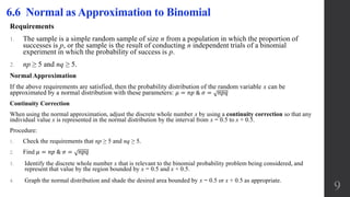
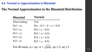
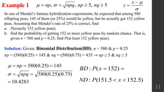
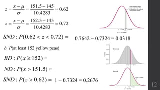
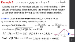
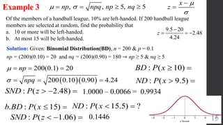
The document discusses approximating binomial probabilities with a normal distribution. It defines the binomial distribution and states the requirements for the normal approximation are that np and nq must both be greater than or equal to 5. The normal approximation involves using a normal distribution with mean np and standard deviation npq. Examples are provided demonstrating how to calculate probabilities for binomial experiments using the normal approximation.

1. Elementary Statistics
Chapter 6:
Normal Probability
Distributions
6.6 Normal as
Approximation to
Binomial
1

2. Chapter 6: Normal Probability Distribution
6.1 The Standard Normal Distribution
6.2 Real Applications of Normal Distributions
6.3 Sampling Distributions and Estimators
6.4 The Central Limit Theorem
6.5 Assessing Normality
6.6 Normal as Approximation to Binomial
2
Objectives:
• Identify distributions as symmetric or skewed.
• Identify the properties of a normal distribution.
• Find the area under the standard normal distribution, given various z values.
• Find probabilities for a normally distributed variable by transforming it into a standard normal variable.
• Find specific data values for given percentages, using the standard normal distribution.
• Use the central limit theorem to solve problems involving sample means for large samples.
• Use the normal approximation to compute probabilities for a binomial variable.

3. Recall: The Standard Normal Distribution
Normal Distribution
If a continuous random variable has a distribution with a graph that
is symmetric and bell-shaped, we say that it has a normal
distribution. The shape and position of the normal distribution
curve depend on two parameters, the mean and the standard
deviation.
SND: 1) Bell-shaped 2) µ = 0 3) σ = 1
3
2 2
( ) (2 )
2
x
e
y
 
 
 

2
1
2
:
2
x
e
OR y


 
 
  
 

x
z




TI Calculator:
Normal Distribution Area
1. 2nd + VARS
2. normalcdf(
3. 4 entries required
4. Left bound, Right
bound, value of the
Mean, Standard
deviation
5. Enter
6. For −∞, 𝒖𝒔𝒆 − 𝟏𝟎𝟎𝟎
7. For ∞, 𝒖𝒔𝒆 𝟏𝟎𝟎𝟎
TI Calculator:
Normal Distribution: find
the Z-score
1. 2nd + VARS
2. invNorm(
3. 3 entries required
4. Left Area, value of the
Mean, Standard
deviation
5. Enter

4. An estimator is a statistic used to infer (or estimate) the value of a population
parameter.
Unbiased Estimator
An unbiased estimator is a statistic that targets the value of the corresponding
population parameter in the sense that the sampling distribution of the statistic has a
mean that is equal to the corresponding population parameter such as:
Proportion: 𝒑
Mean: 𝒙
Variance: s²
Biased Estimator
These statistics are biased estimators. That is, they do not target the value of the
corresponding population parameter:
• Median
• Range
• Standard deviation s
4
Recall: Sampling Distributions and Estimators
x
z





5. Recall: Central Limit Theorem and the Sampling Distribution 𝒙
A sampling distribution of sample means is a distribution obtained by using the means computed from random samples of a
specific size taken from a population. Sampling error is the difference between the sample measure and the corresponding
population measure due to the fact that the sample is not a perfect representation of the population.
The Central Limit Theorem tells us that for a population with any distribution, the distribution of the sample means
approaches a normal distribution as the sample size increases.
1. The random variable x has a distribution (which may or may not be normal) with mean μ and standard deviation σ.
2. Simple random samples all of size n are selected from the population. (The samples are selected so that all possible samples of
the same size n have the same chance of being selected.)
Conclusion:
1. The distribution of sample 𝑥 will, as the sample size increases, approach a normal distribution.
2. The mean of the sample means is the population mean 𝜇 𝑥 = 𝜇 .
3. The standard deviation of all sample means ( also called the standard error of the mean) is 𝜎 𝑥= 𝜎/ 𝑛
1. For samples of size n > 30, the distribution of the sample means can be approximated reasonably well by a normal distribution.
The approximation becomes closer to a normal distribution as the sample size n becomes larger.
2. If the original population is normally distributed, then for any sample size n, the sample means will be normally distributed (not
just the values of n larger than 30).
Requirements: Population has a normal distribution or n > 30:
5/
x
x
x x
z
n
 
 
 
 

6. Key Concept:
Determine whether the requirement of a normal distribution is satisfied:
(1) visual inspection of a histogram to see if it is roughly bell-shaped
(2) identifying any outliers; and
(3) constructing a normal quantile plot.
Normal Quantile Plot
A normal quantile plot (or normal probability plot) is a graph of points (x, y)
where each x value is from the original set of sample data, and each y value is the
corresponding z score that is expected from the standard normal distribution.
Recall: 6.5 Assessing Normality
6
(x, y = Z-score)

7. Key Concept:
Use a normal distribution as an approximation to the binomial probability distribution: BD:
n & p⇾ q = 1 − p
if the conditions of np ≥ 5 and nq ≥ 5 are both satisfied, then probabilities from a binomial probability
distribution can be approximated reasonably well by using a normal distribution having these
parameters: 𝜇 = 𝑛𝑝 & 𝜎 = 𝑛𝑝𝑞
The binomial probability distribution is discrete (with whole numbers for the random variable x), but
the normal approximation is continuous. To compensate, we use a “continuity correction” with a
whole number x represented by the interval from x − 0.5 to x + 0.5.
Recall: A binomial probability distribution has
(1) a fixed number of trials;
(2) trials that are independent;
(3) trials that are each classified into two categories commonly referred to as success and failure;
and
(4) trials with the property that the probability of success remains constant.
6.6 Normal as Approximation to Binomial
7

8. Notation
n = the fixed number of trials
x = the specific number of successes in n trials
p = probability of success in one of the n trials
q = probability of failure in one of the n trials (so q = 1 − p)
Rationale for Using a Normal Approximation:
We saw in a previous section that the sampling distribution of a sample proportion
tends to approximate a normal distribution. Also, see the following probability
histogram for the binomial distribution with n = 580 and p = 0.25. (In one of Mendel’s
famous hybridization experiments, he expected 25% of his 580 peas to be yellow, but
he got 152 yellow peas, for a rate of 26.2%.) The bell-shape of this graph suggests that
we can use a normal distribution to approximate the binomial distribution.
6.6 Normal as Approximation to Binomial
8

9. Requirements
1. The sample is a simple random sample of size n from a population in which the proportion of
successes is p, or the sample is the result of conducting n independent trials of a binomial
experiment in which the probability of success is p.
2. np ≥ 5 and nq ≥ 5.
Normal Approximation
If the above requirements are satisfied, then the probability distribution of the random variable x can be
approximated by a normal distribution with these parameters: 𝜇 = 𝑛𝑝 & 𝜎 = 𝑛𝑝𝑞
Continuity Correction
When using the normal approximation, adjust the discrete whole number x by using a continuity correction so that any
individual value x is represented in the normal distribution by the interval from x − 0.5 to x + 0.5.
Procedure:
1. Check the requirements that np ≥ 5 and nq ≥ 5.
2. Find 𝜇 = 𝑛𝑝 & 𝜎 = 𝑛𝑝𝑞
3. Identify the discrete whole number x that is relevant to the binomial probability problem being considered, and
represent that value by the region bounded by x − 0.5 and x + 0.5.
4. Graph the normal distribution and shade the desired area bounded by x − 0.5 or x + 0.5 as appropriate.
6.6 Normal as Approximation to Binomial
9

10. 6.6 Normal as Approximation to Binomial
The Normal Approximation to the Binomial Distribution
Binomial
When finding:
P(X = a)
P(X  a)
P(X > a)
P(X  a)
P(X < a)
Normal
Use:
P(a – 0.5 < X < a + 0.5)
P(X > a – 0.5)
P(X > a + 0.5)
P(X < a + 0.5)
P(X < a – 0.5)
For all cases, , , 5, 5   np npq np nq 
10

11. 11
In one of Mendel’s famous hybridization experiments, he expected that among 580
offspring peas, 145 of them (or 25%) would be yellow, but he actually got 152 yellow
peas. Assuming that Mendel’s rate of 25% is correct, find
a. P(exactly 152 yellow peas).
b. find the probability of getting 152 or more yellow peas by random chance. That is,
given n = 580 and p = 0.25, find P(at least 152 yellow peas).
Example 1
Solution: Given: Binomial Distribution(BD), n = 580 & p = 0.25
np = (580)(0.25) = 145 & nq = (580)(0.75) = 435 ⇾ np ≥ 5 & nq ≥ 5
580(0.25) 145
580(0.25)(0.75)
10.4283
np
npq


  
 

, , 5, 5np npq np nq    
: ( 152)BD P x  
: (151.5 152.5)ND P x 
x
z





12. 12
151.5 145
0.62
10.4283
x
z


 
  
152.5 145
0.72
10.4283
x
z


 
  
0.7642 − 0.7324 = 0.0318: (0.62 0.72)SND P z  
b. P(at least 152 yellow peas)
: ( 152)BD P x  
: ( 151.5)ND P x  
: ( 0.62)SND P z   1 − 0.7324 = 0.2676

13. Technology for Binomial Probabilities (Statdisk)
13

14. 14
Assume that 6% of American drivers text while driving. If 300
drivers are selected at random, find the probability that exactly
25 say they text while driving. (Use Normal approximation)
Example 2
Solution: Given: Binomial Distribution(BD), n = 300 & p = 0.06
np = (300)(0.06) = 18 ≥ 5 and nq = (300)(0.94) = 282 ≥ 5
  
300(0.06) 18
300 0.06 0.94 4.1134
np
npq


  
  
, , 5, 5np npq np nq    
x
z




: ( 25)BD P x   : (24.5 25.5)ND P x  
24.5 18 25.5 18
1.58, 1.82
4.11 4.11
 
   z z
0.9656 – 0.9429 = 0.0227: (1.58 1.82)SND P z  

15. 15
Of the members of a handball league, 10% are left-handed. If 200 handball league
members are selected at random, find the probability that
a. 10 or more will be left-handed.
b. At most 15 will be left-handed.
Example 3
Solution: Given: Binomial Distribution(BD), n = 200 & p = 0.1
np = (200)(0.10) = 20 and nq = (200)(0.90) = 180 ⇾ np ≥ 5 & nq ≥ 5
  
200(0.1) 20
200 0.10 0.90 4.24
np
npq


  
  
, , 5, 5np npq np nq    
: ( 10)BD P x  
: ( 9.5)ND P x  
x
z




9.5 20
2.48
4.24

  z
: ( 2.48)SND P z    1.0000 – 0.0066 = 0.9934
. : ( 15)b BD P x   : ( 15.5) ?ND P x  
: ( 1.06)SND P z    0.1446