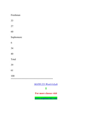
1. (TCO 1) An Input Area (as it applies to Excel 2010) is defined as______. 2. (TCO 1) In Excel 2010, a sheet tab ________. 3. (TCO 1) Which of the following best describes the AutoComplete function? 4. (TCO 1) Which of the following best describes the order of precedence as it applies to math operations in Excel?

1. MATH 221 Week 1 Quiz
For more classes visit
www.snaptutorial.com
1. (TCO 1) An Input Area (as it applies to Excel 2010) is defined
as______.
2. (TCO 1) In Excel 2010, a sheet tab ________.
3. (TCO 1) Which of the following best describes the AutoComplete
function?
4. (TCO 1) Which of the following best describes the order of
precedence as it applies to math operations in Excel?
5. (TCO 1) Which of the following describes the Auto Fill in Excel
2010?
6. (TCO 1) In Excel 2010, a column width ________.
7. (TCO 1) Which of the following best describes a "Range" in Excel
2010?
8. (TCO1) In Excel, a border ________.
9. (TCO 3) A chart can be defined as ________.
10. (TCO 3) A __________ is usually the most effective way to display
proportional relationships, such as market share data, where the
individual data values represent parts of a whole

2. 11. (TCO 3) When creating a chart in Excel, the plot area ________.
12. (TCO 3) To display similar data in a single column, with each series
of data distinguished by a different color, use a:
13. (TCO 3) A pie chart with one or more slices separated for emphasis
is called a(n) ____________ pie chart.
14. (TCO 3) When you select a chart, Excel displays a Chart Tools
contextual tab with three specific tabs:
15. (TCO 3) Which of the following best describes a trendline?
=============================
MATH 221 Week 3 Quiz
For more classes visit
www.snaptutorial.com
1. (TCO 1) What method of data collection would you use to collect data
for a study of the salaries of college professors at a particular college?
2. (TCO 2) There is a relationship between smoking cigarettes and
getting emphysema. This statement describes
3. (TCO 2) The colors of automobiles on a used car lot are
4. (TCO 1) A lobbyist for a major airspace firm assigns a number to
each legislator and then uses a computer to randomly generate ten
numbers. The lobbyist contacts the legislators corresponding to these
numbers. What sampling technique is used?

3. 5. (TCO 2) The average salary of all General Motors workers is $42,500.
This number is a
6. (TCO 2) Subjects in a sample, when properly selected, should possess
7. (TCO 2) Suppose the standard deviation is 13.1. What is the variance?
8. (TCO 10) This data shows the temperatures on randomly chosen days
during a summer class and the number of absences on those days.
(temperature, number of absences) (72, 3), (85, 7), (91, 10), (90, 10),
(88, 8), (98, 15), (75, 4), (100, 16), (80, 5)
Find the equation of the regression line for the given data.
9. (TCO 9) A researcher found a significant relationship between a
person’s age, a, the number of hours a person works per week, b, and the
number of accidents, y, the person has each year. The relationship can be
represented by the multiple regression equation y = -3.2 + 0.012a +
0.23b. Predict the number of accidents per year (to the nearest whole
number) for a person whose age is 45 and who works 42 hours per week
10. (TCO 9) Interpret an r value of -0.82
1. (TCO 3) Use this table to answer the questions.
Height (in inches)
Frequency
50-52
5
53-55

4. 8
56-58
12
59-61
13
62-64
11
1. Identify the class width.
2. Identify the midpoint of the first class.
3. Identify the class boundaries of the first class.
4. Give the relative frequency for each class.
2. (TCO 3) The heights in inches of 18 randomly selected adult males in
LA are listed as: 70, 69, 72, 57, 70, 66, 69, 73, 80, 68, 71, 68, 72, 67, 58,
74, 81, 72.
1. Display the data in a stem-and-leaf plot.
2. Find the mean.3. Find the median.
4. Find the mode.
5. Find the range.
6. Find the variance.
7. Find the standard deviation
Related Tutorials
=============================
MATH 221 Week 5 Quiz

5. For more classes visit
www.snaptutorial.com
1. (TCO 4) How many ways can an EMT union committee of 5 be
chosen from 25 EMTs?
2. (TCO 4) Which of the following cannot be a probability?
3. (TCO 4) List the sample space of rolling a 6 sided die.
4. (TCO 4) What is the probability of choosing a queen on the 2nd draw
if the first was a queen (without replacement)?
5. (TCO 4) A respiratory class has 33 women and 18 men. If a student is
chosen randomly to be the team leader, what is the probability the
student is a woman?
6. (TCO 4) Compute the following: 3! ÷ (0! * 3!)
7. (TCO 5) Decide whether the experiment is a binomial, Poisson, or
neither based on the information given. A car towing service company
averages two calls per hour. We’re interested in knowing the probability
that in a randomly selected hour they will receive a call.
8. (TCO 5) Given a Poisson distribution with mean = 4. Find P(X < 3).
9. (TCO 5) Given the random variable X = {7, 8} with P(7) = 0.7 and
P(8) = 0.3. Find E(X).

6. 10. (TCO 5) If X = {1, 2, 3, 4, 5, 6} and P(1) = 0.2, P(2) = 0.2, P(3) =
0.2, P(4) = 0.2, P(5) = 0.2, and P(6) = 0.2, can distribution of the random
variable X be considered a probability distribution?
11. (TCO 5) If X = {1, 2, 3, 4, 5, 6} and P(1) = 0.3, P(2) = 0.2, P(3) =
0.1, P(4) = 0.1, P(5) = 0.1, and P(6) = 0.3, can distribution of the random
variable X be considered a probability distribution?
12. (TCO 5) The weight of a box of Cheerios represents what kind of
distribution?
13. (TCO 5) Your baby’s weight represents what kind of distribution?
14. (TCO 5) The number of patients donating blood in a day represents
what kind of distribution?
1. (TCO 5) We have a binomial experiment with p = 0.6 and n = 2.
(1) Set up the probability distribution by showing all x values and their
associated probabilities.
(2) Compute the mean, variance, and standard deviation
2. (TCO 4) What is the probability that the student carries a credit card
given he's a sophomore?
Class
Credit Card Carrier
Not a Credit Card Carrier
Total
Freshman

7. 33
27
60
Sophomore
6
34
40
Total
39
61
100
3. (TCO 4) Some students were asked if they carry a credit card. Here
are their responses.
Class
Credit Card Carrier
Not a Credit Card Carrier
Total
Freshman

8. 33
27
60
Sophomore
6
34
40
Total
39
61
100
What is the probability that the student is a sophomore?
4. (TCO 4) What is the probability that the student is a sophomore and
doesn't carry a credit card?
Class
Credit Card Carrier
Not a Credit Card Carrier
Total

9. Freshman
33
27
60
Sophomore
6
34
40
Total
39
61
100
===============================
MATH 221 Week 6 iLab
For more classes visit
www.snaptutorial.com

10. Name:
Statistical Concepts:
· Data Simulation
· Confidence Intervals
· Normal Probabilities
Short Answer Writing Assignment
All answers should be complete sentences.
We need to find the confidence interval for the SLEEP variable. To do
this, we need to find the mean and then find the maximum error. Then
we can use a calculator to find the interval, (x – E, x + E).
First, find the mean. Under that column, in cell E37,
type=AVERAGE(E2:E36). Under that in cell E38, type
=STDEV(E2:E36). Now we can find the maximum error of the
confidence interval. To find the maximum error, we use the
“confidence” formula. In cell E39,
type=CONFIDENCE.NORM(0.05,E38,35). The 0.05 is based on the
confidence level of 95%, the E38 is the standard deviation, and 35 is the
number in our sample. You then need to calculate the confidence
interval by using a calculator to subtract the maximum error from the
mean (x-E) and add it to the mean (x+E).
1. Give and interpret the 95% confidence interval for the hours of sleep a
student gets.
2. Give and interpret the 99% confidence interval for the hours of sleep a
student gets.

11. 3. Compare the 95% and 99% confidence intervals for the hours of sleep
a student gets. Explain the difference between these intervals and why
this difference occurs.
In the week 2 lab, you found the mean and the standard deviation for the
HEIGHT variable for both males and females. Use those values for
follow these directions to calculate the numbers again.
(From week 2 lab: Calculate descriptive statistics for the variable Height
by Gender. Click on Insert and then Pivot Table. Click in the top box
and select all the data (including labels) from Height through Gender.
Also click on “new worksheet” and then OK. On the right of the new
sheet, click on Height and Gender, making sure that Gender is in
theRows box and Height is in the Values box. Click on the down arrow
next to Height in the Values box and select Value Field Settings. In the
pop up box, click Average then OK. Write these down. Then click on
the down arrow next to Height in the Values box again and select Value
Field Settings. In the pop up box, click on StdDev then OK. Write these
values down.)
You will also need the number of males and the number of females in
the dataset. You can either use the same pivot table created above by
selecting Count in the Value Field Settings, or you can actually count in
the dataset.
Then in Excel (somewhere on the data file or in a blank worksheet),
calculate the maximum error for the females and the maximum error for
the males. To find the maximum error for the females,
type=CONFIDENCE.T(0.05,stdev,#), using the females’ height standard
deviation for “stdev” in the formula and the number of females in your
sample for the “#”. Then you can use a calculator to add and subtract
this maximum error from the average female height for the 95%
confidence interval. Do this again with 0.01 as the alpha in the
beginning of the formula to find the 99% confidence interval.

12. Find these same two intervals for the male data by using the same
formula, but using the males’ standard deviation for “stdev” and the
number of males in your sample for the “#”.
4. Give and interpret the 95% confidence intervals for males and females
on the HEIGHT variable. Which is wider and why?
5. Give and interpret the 99% confidence intervals for males and females
on the HEIGHT variable. Which is wider and why?
6. Find the mean and standard deviation of the DRIVE variable by using
=AVERAGE(A2:A36) and =STDEV(A2:A36). Assuming that this
variable is normally distributed, what percentage of data would you
predict would be less than 40 miles? This would be based on the
calculated probability. Use the formula =NORM.DIST(40, mean,
stdev,TRUE). Now determine the percentage of data points in the
dataset that fall within this range. To find the actual percentage in the
dataset, sort the DRIVE variable and count how many of the data points
are less than 40 out of the total 35 data points. That is the actual
percentage. How does this compare with your prediction?
7. What percentage of data would you predict would be between 40 and
70 and what percentage would you predict would be more than 70
miles? Subtract the probabilities found through =NORM.DIST(70,
mean, stdev, TRUE) and =NORM.DIST(40, mean, stdev, TRUE) for the
“between” probability. To get the probability of over 70, use the same
=NORM.DIST(70, mean, stdev, TRUE) and then subtract the result
from 1 to get “more than”. Now determine the percentage of data points
in the dataset that fall within this range, using same strategy as above for
counting data points in the data set. How do each of these compare with
your prediction and why is there a difference?
============================