Downloaded 129 times


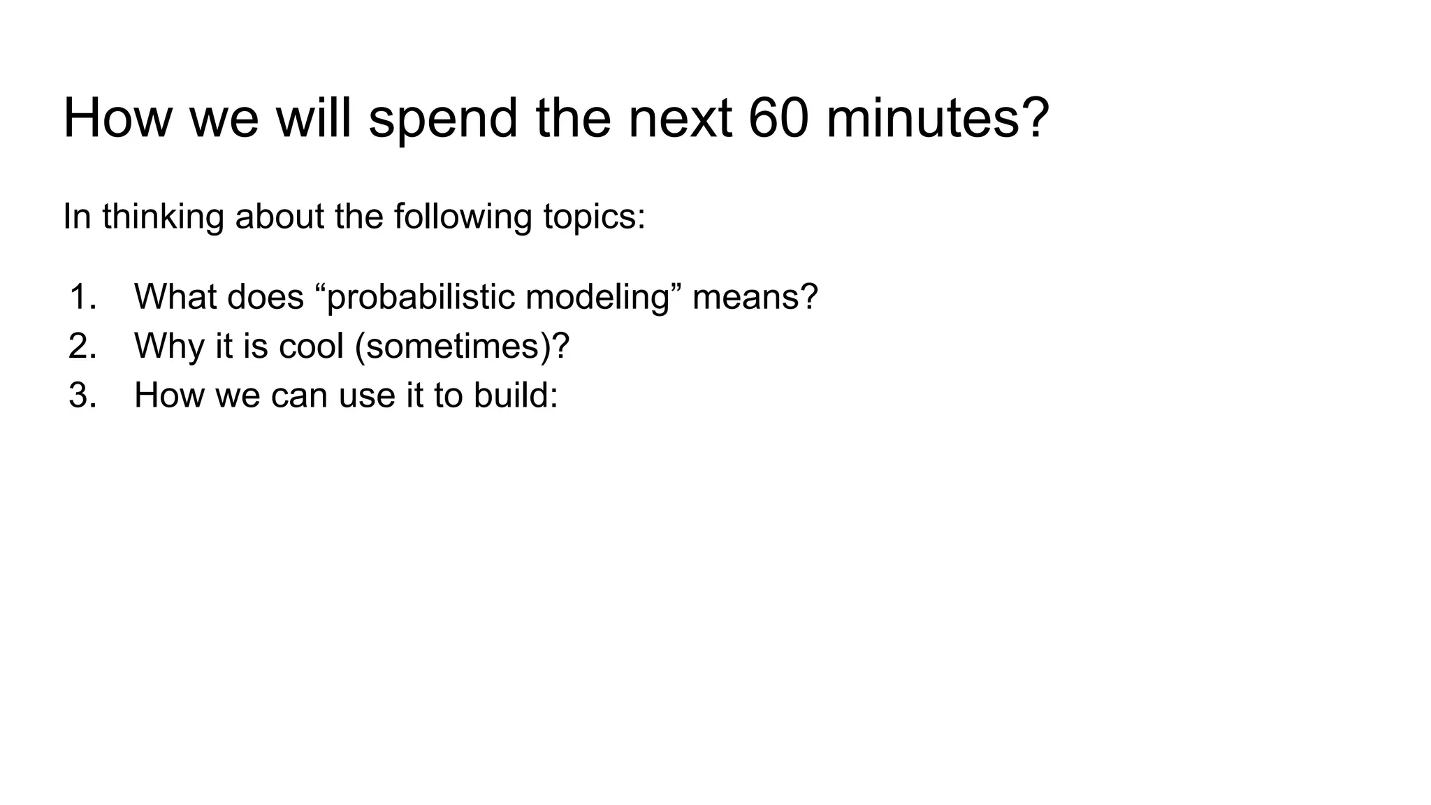


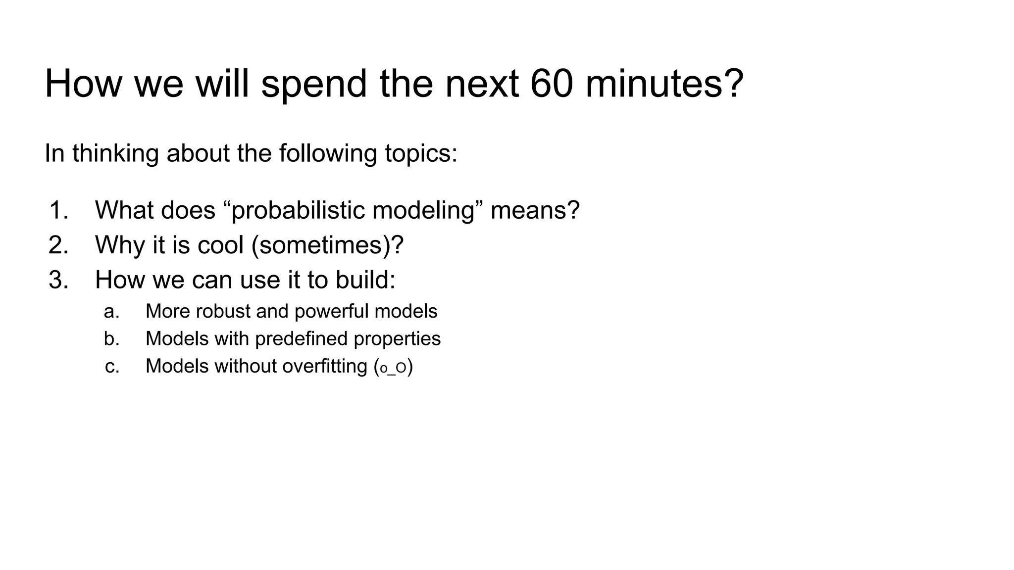


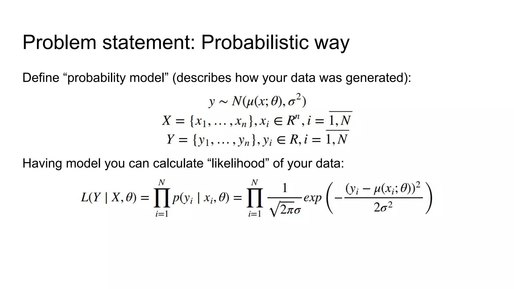
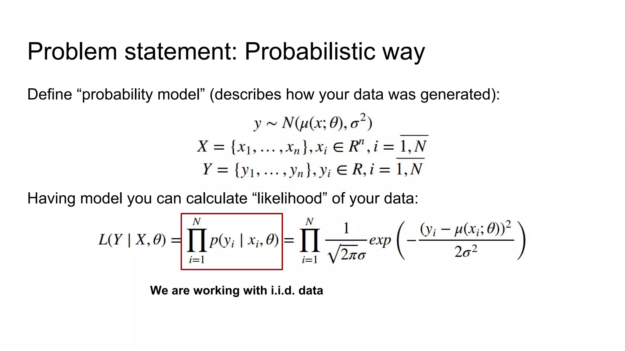
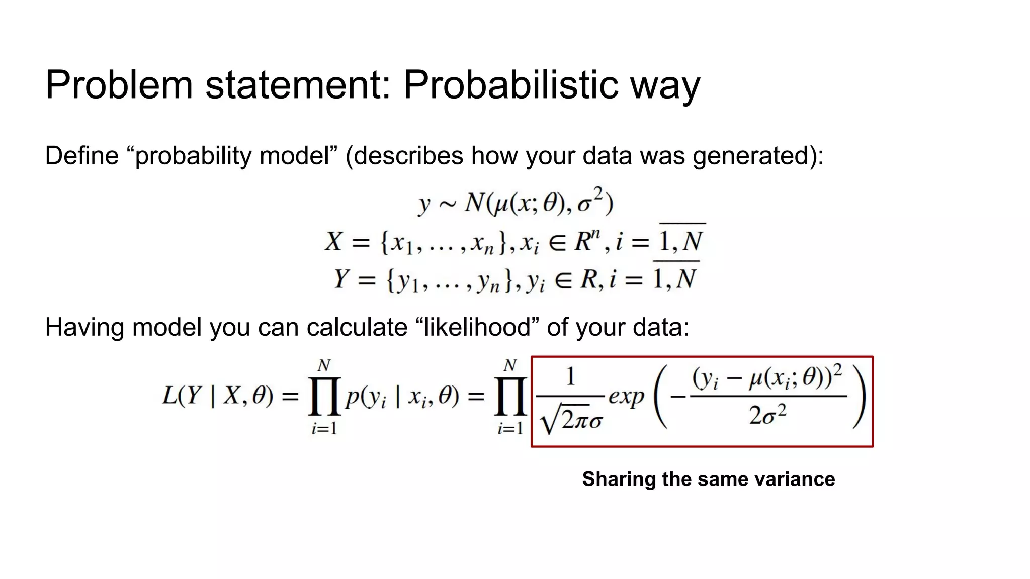
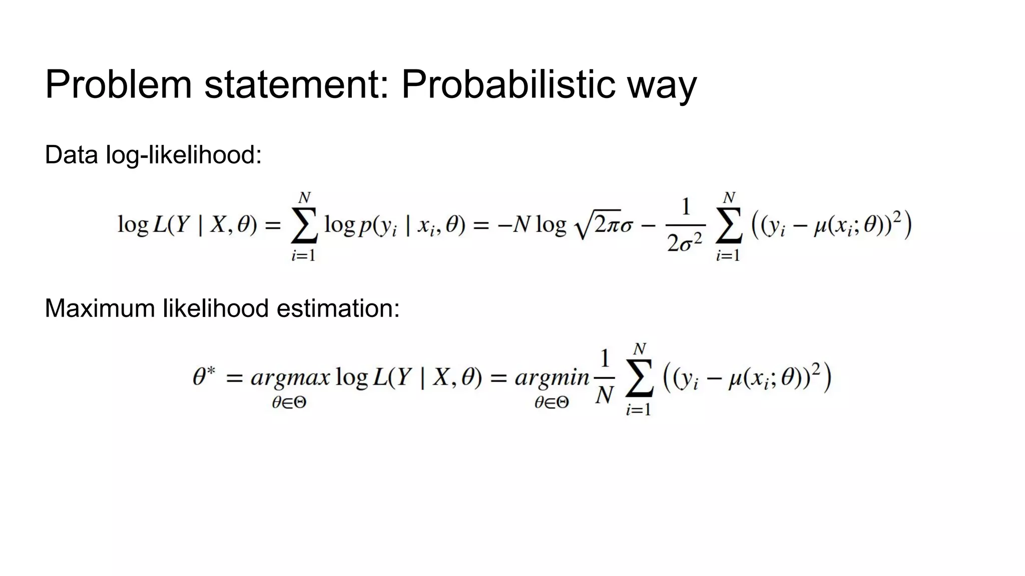


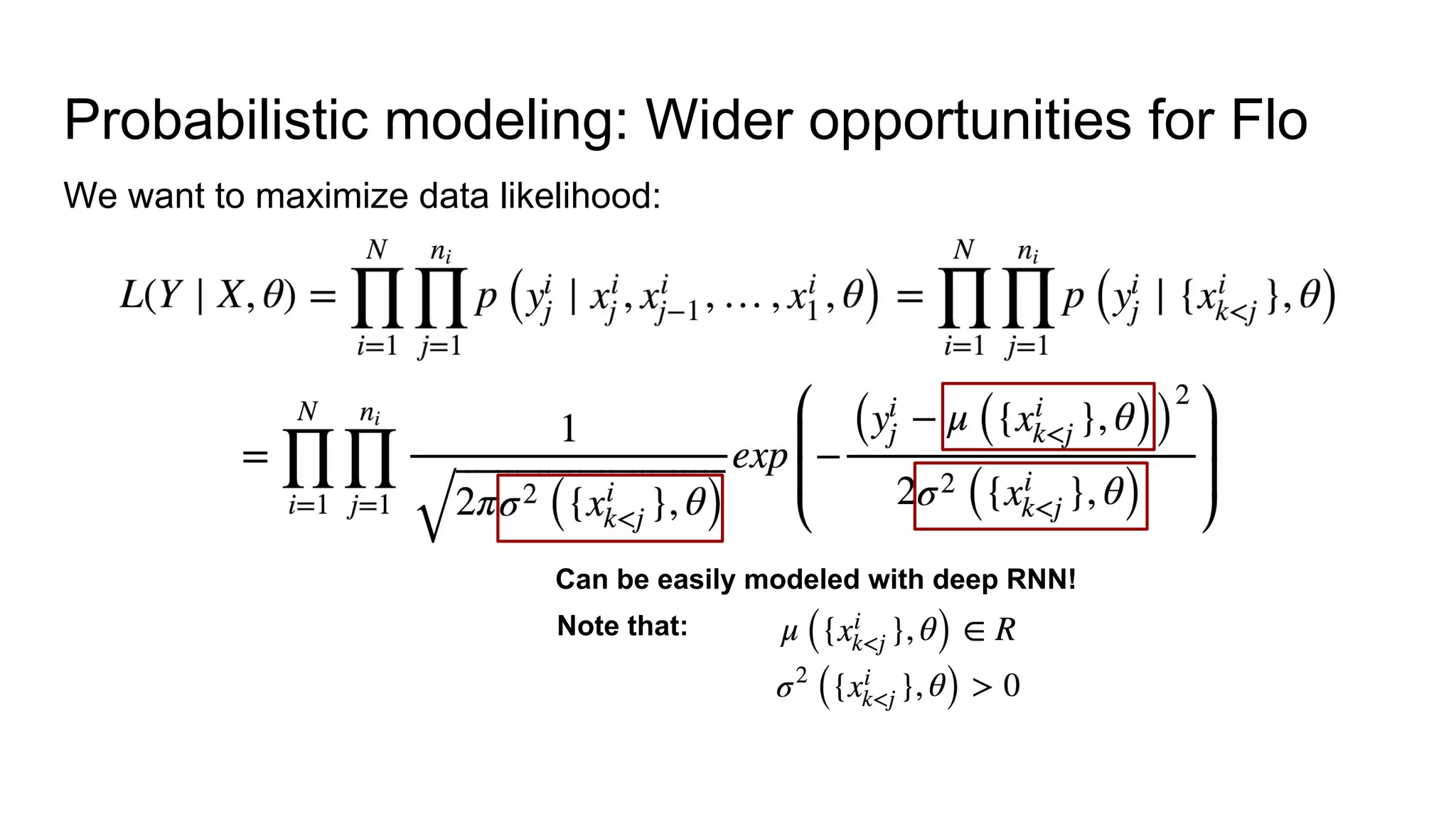
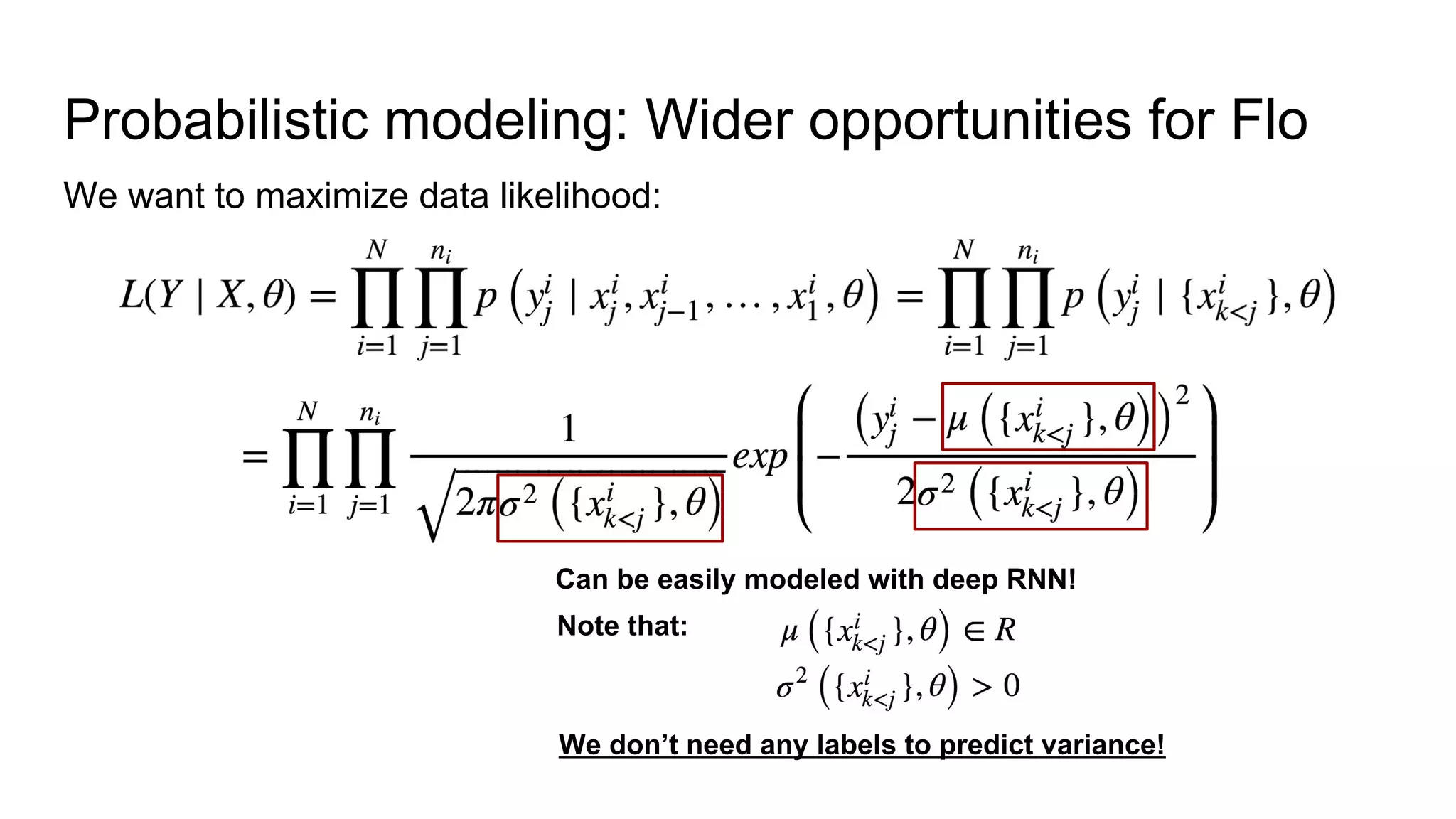


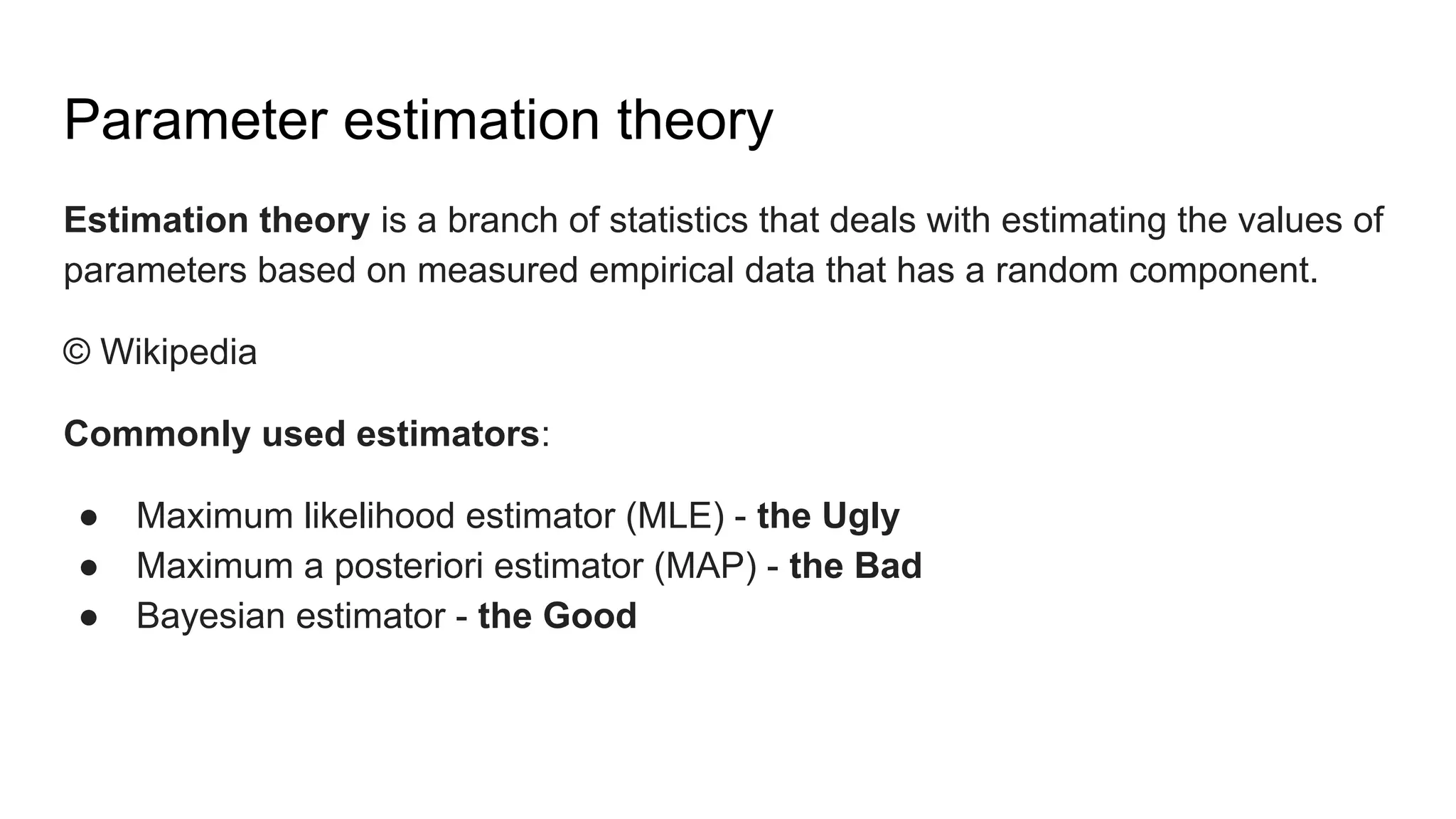

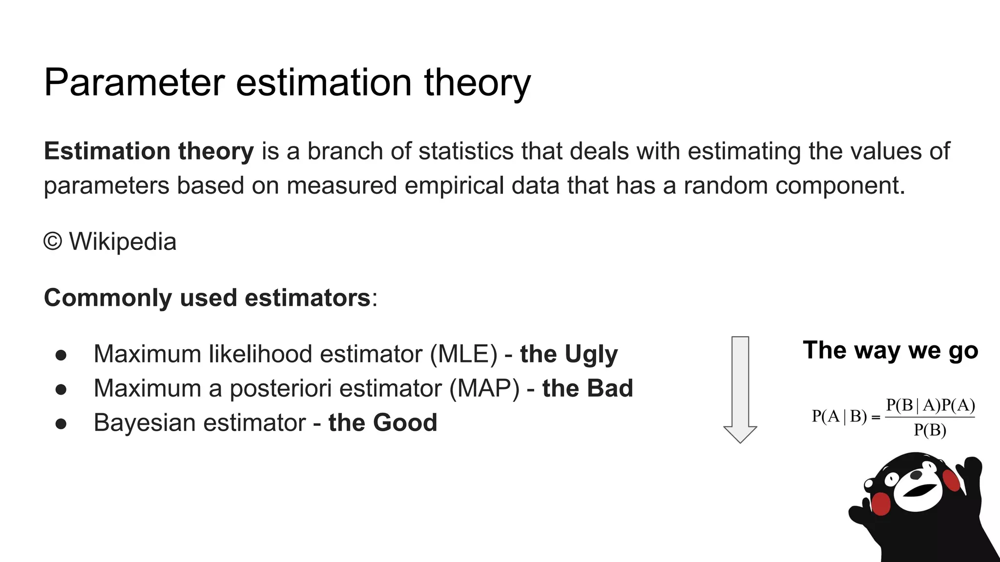


The document discusses probabilistic modeling in deep learning. It will cover: 1. What probabilistic modeling means and why it is useful. 2. How probabilistic modeling can be used to build more robust models, models with predefined properties, models without overfitting, and infinite ensembles of models. 3. Examples of how probabilistic modeling provides wider opportunities than empirical modeling by allowing the modeling of distributions and uncertainties rather than just point estimates. This includes using probabilistic modeling with deep RNNs to predict distributions over cycle lengths based on user state time series.


![ict_presentation_final_final_final[1].pptx](https://cdn.slidesharecdn.com/ss_thumbnails/ictpresentationfinalfinalfinal1-251230145259-2b4839bd-thumbnail.jpg?width=640&height=640&fit=bounds)


